Cartoon-texture oscillation decomposition demo

Cartoon-texture oscillation decomposition demo#

Problem setting#

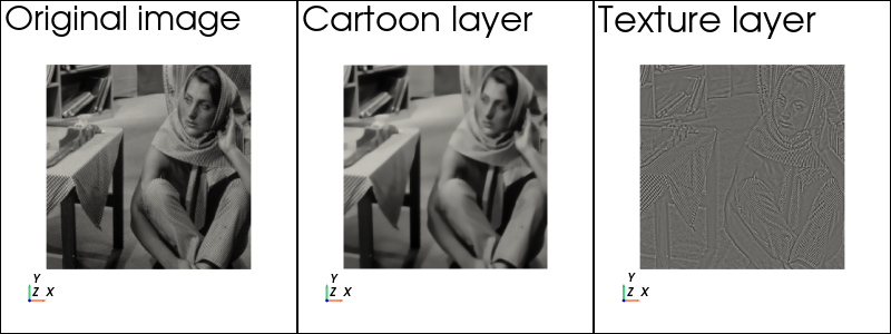
We consider an image processing problem which consists in decomposing an image \(y=u+v\) into a cartoon-like component \(u\) and a texture component \(v\) (here we assume that the image is not noisy). The cartoon layer \(u\) captures flat regions separated by sharp edges, whereas the texture component \(v\) contains the high frequency oscillations. There are many existing models to perform such a decomposition, in the following, we implement the model proposed by Y. Meyer [Meyer, 2001]: \(\newcommand{\dOm}{\,\text{d}\Omega}\newcommand{\div}{\operatorname{div}}\)

\[\begin{split}\begin{array}{rl} \displaystyle{\inf_{u,v}} & \displaystyle{\int_\Omega \|\nabla u\|_2 \dOm + \alpha \|v\|_G} \\ \text{s.t.} & y=u+v \\ \\ \text{where} & \displaystyle{\|v\|_G = \inf_{\boldsymbol{g}\in L^{\infty}(\Omega;\mathbb{R}^2)} \left\{\left\|\sqrt{g_1^2+g_2^2}\right\|_{\infty} \text{ s.t. } v=\div \boldsymbol{g}\right\}} \end{array} \end{split}\]

This model favors flat regions in \(u\) due to the use of the TV norm and oscillatory regions in \(v\) since \(\|v\|_G\) increases for characteristic functions. Following [Weiss et al., 2009], we reformulate the model as:

\[\begin{split}\begin{array}{rl} \displaystyle{\inf_{u,\boldsymbol{g}}} & \displaystyle{\int_\Omega \|\nabla u\|_2 \dOm} \\ \text{s.t.} & y=u+\div(\boldsymbol{g}) \\ & \sqrt{g_1^2+g_2^2}\leq \alpha \end{array} \end{split}\]

Implementation#

After importing the relevant packages, we first load the input image.

import matplotlib.pyplot as plt
from matplotlib import rcParams
from pathlib import Path
import pyvista as pv
import numpy as np
from mpi4py import MPI
import ufl
from dolfinx import mesh, fem, geometry, plot
from dolfinx_optim.mosek_io import MosekProblem
from dolfinx_optim.convex_function import L2Norm, L2Ball

path = Path(".")

image = plt.imread(path / "Barbara_256x256.png")
image = image[::-1, :]
Nx, Ny = image.shape
xx = np.arange(Nx + 1)
yy = np.arange(Ny + 1)
xx = (xx[1:] + xx[:-1]) / 2.0 / Nx
yy = (yy[1:] + yy[:-1]) / 2.0 / Ny
x, y = np.meshgrid(xx, yy)
x = x.ravel()
y = y.ravel()
z = np.zeros_like(x)
points = np.vstack((x, y, z)).T

We first represent this image as a DG0 field defined on a quadrilateral mesh of size \(N\times N\).

domain0 = mesh.create_unit_square(
    MPI.COMM_WORLD, Nx, Ny, cell_type=mesh.CellType.quadrilateral
)
bb_tree = geometry.bb_tree(domain0, domain0.topology.dim)
cell_candidates = geometry.compute_collisions_points(bb_tree, points)  # get candidates
colliding_cells = geometry.compute_colliding_cells(
    domain0, cell_candidates, points
)  # get actual
# represent image as DG0 on quad mesh
V00 = fem.functionspace(domain0, ("DG", 0))
y0 = fem.Function(V00)
cells = [c for i in range(len(colliding_cells)) for c in colliding_cells.links(i)]
y0.x.array[cells] = image.ravel()

We will then use a Crouzeix-Raviart interpolation for \(u\) and a Raviart-Thomas interpolation for \(\boldsymbol{g}\). As those function spaces are defined on triangular meshes only, we define a new triangular mesh and interpolate the quad DG0 field on a triangular DG0 mesh.

domain = mesh.create_unit_square(
    MPI.COMM_WORLD, Nx, Ny, cell_type=mesh.CellType.triangle
)

V0 = fem.functionspace(domain, ("DG", 0))
y = fem.Function(V0)

# create non-matching meshes interpolation data
fine_mesh_cell_map = domain.topology.index_map(domain.topology.dim)
num_cells_on_proc = fine_mesh_cell_map.size_local + fine_mesh_cell_map.num_ghosts
cells = np.arange(num_cells_on_proc, dtype=np.int32)
interpolation_data = fem.create_nonmatching_meshes_interpolation_data(
    V0.mesh.geometry, V0.element, V00.mesh, cells, padding=1e-14
)
# interpolate on non-matching mesh
y.interpolate(y0, nmm_interpolation_data=interpolation_data)

We now define the variational problem by creating the two optimization variables \(u\) and \(\boldsymbol{g}\).

prob = MosekProblem(domain, "Cartoon/texture decomposition")
Vu = fem.functionspace(domain, ("CR", 1))
Vg = fem.functionspace(domain, ("RT", 1))

u, g = prob.add_var([Vu, Vg], name=["Cartoon", "Texture"])

The constraint \( y=u+\div(\boldsymbol{g})\) is enforced weakly on the CR space. The implementation reads as:

lamb_ = ufl.TestFunction(Vu)
constraint = ufl.dot(lamb_, u + ufl.div(g)) * ufl.dx
rhs = ufl.dot(lamb_, y) * ufl.dx
prob.add_eq_constraint(constraint, b=rhs)

We then add the TV-norm objective constraint and the G-norm constraint.

alpha = fem.Constant(domain, 2e-4)

tv_norm = L2Norm(ufl.grad(u), 1)
prob.add_convex_term(tv_norm)

g_norm = L2Ball(g / alpha, 2)
prob.add_convex_term(g_norm)

We now optimize the problem. For plotting, we interpolate the cartoon part on the DG0 space.

prob.parameters["log_level"]=0
prob.optimize()

u0 = fem.Function(V0)
u0.interpolate(u)

We finally plot the result using pyvista.

../../_images/388eadb0ac95f74fedf6dfc3c2138f75b1b6683bc99e26a5cb864eb94d3db1c8.png

References#

[Mey01]

Yves Meyer. Oscillating patterns in image processing and nonlinear evolution equations: the fifteenth Dean Jacqueline B. Lewis memorial lectures. Volume 22. American Mathematical Soc., 2001.

[WBFeraudA09]

Pierre Weiss, Laure Blanc-Féraud, and Gilles Aubert. Efficient schemes for total variation minimization under constraints in image processing. SIAM journal on Scientific Computing, 31(3):2047–2080, 2009.

Cartoon-texture oscillation decomposition demo

Contents

Cartoon-texture oscillation decomposition demo#

Problem setting#

Implementation#

References#