Viscoplastic fluid

Viscoplastic or yield-stress fluids are a particular class of non-Newtonian fluids which behave like a standard Newtonian fluid only if the local stress reaches a critical threshold, the fluid yield stress \(\tau_0\). If the stress is below \(\tau_0\), the fluid behaves like a rigid solid. Such fluids occur in many industrial applications such as civil engineering (fresh concrete), petroleum or cosmetics (crude oil, toothpaste, foams, mayonnaise), natural hazards (lava, muds), etc. One of the most simple model to describe such fluids is the Bingham model which assumes a linear Newtonian behavior, characterized by a viscosity \(\mu\), above the yield stress. For recent reviews on yield stress fluids, we refer to [Balmforth et al., 2014, Coussot, 2017].

There numerical resolution is notoriously difficult due to the non-smooth character of their behavior and of the underlying variational principle. Here, we show how computing such flows can be achieved using conic programming and interior-point solvers, for more details see [Bleyer, 2018, Bleyer et al., 2015]. \(\newcommand{\bu}{\boldsymbol{u}}\newcommand{\be}{\boldsymbol{e}}\newcommand{\bd}{\boldsymbol{d}}\newcommand{\bf}{\boldsymbol{f}}\newcommand{\dOm}{\,\text{d}\Omega}\newcommand{\bD}{\boldsymbol{D}}\)

Variational principle

In the case of a steady-state flow under a body force \(\boldsymbol{f}\), the solution velocity field \(\bu\) is obtained from the following minimum principle:

\[\begin{split}\begin{array}{rl} \displaystyle{\min_{\bu}} & \displaystyle{\int_{\Omega} \phi(\bd)\dOm - \int_{\Omega}\boldsymbol{f}\cdot\bu\dOm}\\ \text{s.t.} & \bd = \text{sym}(\nabla \bu)\\ & \operatorname{div}\bu = 0 \end{array}\end{split}\]

where \(\phi(\bd)\) is the dissipation potential corresponding to the material. In the case of a Bingham material characterized by a viscosity \(\mu\) and a yield stress \(\tau_0\), the potential is given by:

\[\begin{equation*} \phi(\bd) = \mu\bd:\bd + \sqrt{2}\tau_0 \sqrt{\bd:\bd} \end{equation*}\]

Note

For a Herschel-Bulkley fluid, the viscous part is a power-law characterized by a viscosity coefficient \(K\) and an exponent \(m\). The potential is given by:

\[\begin{equation*} \phi(\bd) = \dfrac{K}{m+1}2^{(m+1)/2}\|\bd\|^{m+1} + \sqrt{2}\tau_0 \sqrt{\bd:\bd} \end{equation*}\]

Implementation

We consider the problem of a lid-driven square cavity. No slip boundary conditions are enforced on all boundaries except on the top boundary on which a uniform velocity \(\bu=\be_x\) is imposed.

We first import the relevant modules and create a square mesh.

import numpy as np
import matplotlib.pyplot as plt
from pathlib import Path
from mpi4py import MPI
from dolfinx import fem, mesh
import ufl
from dolfinx_optim.mosek_io import MosekProblem
from dolfinx_optim.convex_function import QuadraticTerm, L2Norm

path = Path(".")

N = 75
domain = mesh.create_unit_square(
    MPI.COMM_WORLD, N, N, diagonal=mesh.DiagonalType.crossed
)

We define no-slip boundary conditions on the bottom and lateral sides and impose a unit horizontal velocity \(\bu=\be_x\) on the top boundary.

# get top boundary and remaining part of the cavity
def sides(x):
    return np.isclose(x[0], 0.0) | np.isclose(x[0], 1.0) | np.isclose(x[1], 0)


def top(x):
    return np.isclose(x[1], 1.0) & (x[0] > 0.01) & (x[0] < 0.99)


def middle(x):
    return np.isclose(x[0], 0.5)



# P2 interpolation for velocity
V = fem.functionspace(domain, ("P", 2, (2,)))
side_dofs = fem.locate_dofs_geometrical(V, sides)
top_dofs = fem.locate_dofs_geometrical(V, top)
Vx, _ = V.sub(0).collapse()
middle_dofs = fem.locate_dofs_geometrical((V.sub(0), Vx), middle)[1]


bc = [
    fem.dirichletbc(fem.Constant(domain, (1.0, 0.0)), top_dofs, V),
    fem.dirichletbc(fem.Constant(domain, (0.0, 0.0)), side_dofs, V),
]

We now start defining the optimization problem by adding the velocity \(\bu\) as an optimization variable on a \(\mathbb{P}_2\) function space, constrained to the previously defined boundary conditions. We also enforce the mass conservation condition by adding the following constraint:

\[ \int_\Omega p\:\operatorname{div}(\bu)\: \dOm = 0 \quad \forall p\in V_p \]

where \(V_p\) is the pressure space for pressure test functions \(p\) (used here as Lagrange multipliers). We use a Lagrange \(\mathbb{P}_1\) function space for its discretization, thereby corresponding to a Taylor-Hood mixed formulation.

prob = MosekProblem(domain, "Viscoplastic fluid")

u = prob.add_var(V, bc=bc)

# mass conservation condition
# P1 interpolation for pressure (Lagrange multiplier)
Vp = fem.functionspace(domain, ("P", 1))
p = ufl.TestFunction(Vp)
mass_conserv = p * ufl.div(u) * ufl.dx
prob.add_eq_constraint(mass_conserv)

We now define the fluid viscosity \(\mu\) and yield stress \(\tau_0\). The Bingham number \(\text{Bi}=\tau_0 L/\mu V\) represents the proportion of plastic behavior with respect to the viscous behavior. We also introduce a vector representation for the strain rate field such that:

\[ \|\boldsymbol{d}\|_2^2 = \sum d_i^2 = \bD:\bD=D_{ij}D_{ij} \]

where \(\bD=\text{sym}(\nabla \bu)\) the strain rate tensor and \(\boldsymbol{d}\) its vectorial representation. We then define the viscous potential \(\mu\bD:\bD\) with a QuadraticTerm and the plastic potential \(\sqrt{2}\tau_0\sqrt{\bD:\bD}\) with a L2Norm.

mu, tau0 = fem.Constant(domain, 1.0), fem.Constant(domain, 20.0)

def strain(v):
    D = ufl.sym(ufl.grad(v))
    return ufl.as_vector([D[0, 0], D[1, 1], ufl.sqrt(2) * D[0, 1]])


visc = QuadraticTerm(strain(u), 2)
plast = L2Norm(strain(u), 2)

# add viscous term mu*||strain||_2^2 (factor 2 because 1/2 in QuadraticTerm)
prob.add_convex_term(2 * mu * visc)
# add plastic term sqrt(2)*tau0*||strain||_2
prob.add_convex_term(np.sqrt(2) * tau0 * plast)

The problem is then solved. Note that we slightly relax the default solver tolerance.

prob.parameters["log_level"] = 0 # deactivate solver output
prob.parameters["tol_rel_gap"] = 1e-6
prob.optimize()

(36.88606848632506, 36.84887757188724)

We plot the resulting velocity contour lines

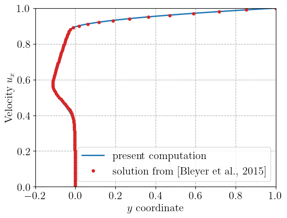
We finally compare the horizontal velocity profile against previous solutions for some Bingham numbers along vertical line \(x=0.5\).

plt.figure()
ux = u.sub(0).collapse()
ux_vals = ux.x.array[middle_dofs]
y_dofs = Vx.tabulate_dof_coordinates()[middle_dofs, 1]
plt.plot(ux_vals, y_dofs, label="present computation")
Bi = int(float(tau0 / mu))
Bi_data_values = [0, 2, 5, 20]
try:
    i = Bi_data_values.index(Bi)
    data = np.loadtxt(path / "viscoplastic_data.csv", skiprows=1)
    plt.plot(
        data[:, i + 1],
        data[:, 0],
        "oC3",
        markersize=4,
        label="solution from [Bleyer et al., 2015]",
    )
except ValueError:
    pass
plt.legend()
plt.xlabel("$y$ coordinate")
plt.ylabel("Velocity $u_x$")
plt.show()

References

[BFO14]

Neil J Balmforth, Ian A Frigaard, and Guillaume Ovarlez. Yielding to stress: recent developments in viscoplastic fluid mechanics. Annual review of fluid mechanics, 46:121–146, 2014.

[Ble18]

Jeremy Bleyer. Advances in the simulation of viscoplastic fluid flows using interior-point methods. Computer Methods in Applied Mechanics and Engineering, 330:368–394, 2018.

[BMDBC15]

Jeremy Bleyer, Mathilde Maillard, Patrick De Buhan, and Philippe Coussot. Efficient numerical computations of yield stress fluid flows using second-order cone programming. Computer Methods in Applied Mechanics and Engineering, 283:599–614, 2015.

[Cou17]

Philippe Coussot. Bingham’s heritage. Rheologica Acta, 56:163–176, 2017.