Elastoplasticity with exponential isotropic hardening#
\(\newcommand{\beps}{\boldsymbol{\varepsilon}} \newcommand{\bepsp}{\boldsymbol{\varepsilon}^\text{p}} \newcommand{\Depsp}{\Delta\boldsymbol{\varepsilon}^\text{p}} \newcommand{\bepsel}{\boldsymbol{\varepsilon}^\text{el}} \newcommand{\bu}{\boldsymbol{u}} \newcommand{\CC}{\mathbb{C}} \newcommand{\KK}{\mathbb{K}} \newcommand{\JJ}{\mathbb{J}} \newcommand{\RR}{\mathbb{R}} \newcommand{\Kk}{\mathcal{K}} \newcommand{\tr}{\operatorname{tr}} \newcommand{\dev}{\operatorname{dev}} \newcommand{\bf}{\boldsymbol{f}} \newcommand{\dOm}{\text{d}\Omega} \DeclareMathOperator*{argmin}{arg\min} \newcommand{\bC}{\boldsymbol{C}} \newcommand{\bQ}{\boldsymbol{Q}} \newcommand{\bx}{\boldsymbol{x}} \newcommand{\T}{^\text{T}}\)
In this demo, we show how to formulate an elastoplastic problem using an incremental variational formulation. We particularize the behavior to a plane strain von Mises yield criterion and an exponential isotropic hardening.
Free-energy and dissipation potential#
In the framework of generalized standard materials [Halphen and Nguyen, 1975], the considered constitutive model is described by:
a choice of state variables consisting of the total strain \(\beps\), the plastic strain \(\bepsp\) and the cumulated equivalent plastic strain \(p\);
its free energy density \(\psi\) consisting of a stored elastic and hardening potentials:
its dissipation potential \(\phi(\dot{\bepsp},\dot{p})\)
We will assume isotropic linear elasticity:
where \(\kappa\) is the compressibility modulus, \(\mu\) the shear modulus and \(\dev(\beps^\text{el})\) the deviatoric elastic strain. Note that splitting the elastic energy into spherical and deviatoric components will later prove useful for the conic reformulation
The hardening potential is assumed to be of exponential type as follows:
where \(\sigma_0\) (resp. \(\sigma_u\)) is the initial (resp. ultimate) yield strength and \(\omega\) a saturation parameter.
Finally, we assume a \(J_2\)-plasticity dissipation potential:
Note that we included in the above the link between the scalar cumulated plastic strain rate and the plastic strain rate tensor \(\dot{p}=\sqrt{\frac{2}{3}}\|\dot{\bepsp}\|\) which will later slightly be reformulated in conic form.
Incremental pseudo-potential#
It can be shown that the solution at time \(t_{n+1}\) in terms of displacement \(\bu\), plastic strain \(\bepsp\) and cumulated plastic strain \(p\) can be obtained as the solution to the following minimization principle [Ortiz and Stainier, 1999]:
where \(\beps = \nabla^s\bu\), \(\mathcal{P}_\text{ext}\) is the power of external loads which we assume to consist only of fixed body forces \(\bf_{n+1}\) on the time step.
Further introducing a backward-Euler approximation for the plastic strain variables evolution :
where \(\Depsp = \bepsp-\bepsp_n\) and \(\Delta p=p-p_n\), we have:
which is a variational problem involving an incremental pseudo-potential:
in which the time increment \(\Delta t\) disappears since the behavior is rate-independent (\(\phi\) being a positively homogeneous convex function).
Mesh generation#
We start by importing the relevant packages and functions we will use.
import matplotlib.pyplot as plt
import numpy as np
from mpi4py import MPI
import ufl
from dolfinx import mesh, fem, io
from dolfinx_optim.mosek_io import MosekProblem
from dolfinx_optim.convex_function import ConvexTerm, QuadraticTerm
from dolfinx_optim.cones import Quad, Exp
from dolfinx_optim.utils import tail, concatenate, to_vect
We create a rectangular plate with two circular notches on its sides using gmsh Python API.
Show code cell source
def generate_notched_plate(W, H, R, mesh_size):
    import gmsh
    from dolfinx.io.gmshio import model_to_mesh

    gmsh.initialize()
    gmsh.option.setNumber("General.Terminal", 0)  # to disable meshing info

    gdim = 2
    mesh_comm = MPI.COMM_WORLD
    model_rank = 0
    if mesh_comm.rank == model_rank:
        rectangle = gmsh.model.occ.addRectangle(0, 0, 0, W, H, tag=1)
        hole1 = gmsh.model.occ.addDisk(
            0,
            H / 2,
            0,
            R,
            R,
            zAxis=[0, 0, 1],
            xAxis=[0.0, 1.0, 0.0],
        )
        hole2 = gmsh.model.occ.addDisk(
            W,
            H / 2,
            0,
            R,
            R,
            zAxis=[0, 0, 1],
            xAxis=[0.0, 1.0, 0.0],
        )
        gmsh.model.occ.cut([(gdim, rectangle)], [(gdim, hole1), (gdim, hole2)])
        gmsh.model.occ.synchronize()

        volumes = gmsh.model.getEntities(gdim)
        gmsh.model.addPhysicalGroup(gdim, [volumes[0][1]], 1, name="Plate")
        gmsh.model.addPhysicalGroup(gdim-1, [8], 1, name="Bottom")
        gmsh.model.addPhysicalGroup(gdim-1, [4], 2, name="Top")

        try:
            field_tag = gmsh.model.mesh.field.add("Box")
            gmsh.model.mesh.field.setNumber(field_tag, "VIn", min(mesh_size))
            gmsh.model.mesh.field.setNumber(field_tag, "VOut", max(mesh_size))
            gmsh.model.mesh.field.setNumber(field_tag, "XMin", 0)
            gmsh.model.mesh.field.setNumber(field_tag, "XMax", W)
            gmsh.model.mesh.field.setNumber(field_tag, "YMin", H / 2 - 0.5 * R)
            gmsh.model.mesh.field.setNumber(field_tag, "YMax", H / 2 + 0.5 * R)
            gmsh.model.mesh.field.setNumber(field_tag, "Thickness", R)
            gmsh.model.mesh.field.setAsBackgroundMesh(field_tag)
        except:
            gmsh.option.setNumber("Mesh.CharacteristicLengthMin", mesh_size)
            gmsh.option.setNumber("Mesh.CharacteristicLengthMax", mesh_size)

        gmsh.model.mesh.generate(gdim)

        domain, markers, facets = model_to_mesh(
            gmsh.model,
            mesh_comm,
            model_rank,
            gdim=gdim,
        )

    gmsh.finalize()
    return domain, markers, facets
We generate the mesh and define the different physical constants for the problem.
R = 0.2
W = 4*R
H = 16*R
mesh_sizes = [0.15, 0.015]
domain, markers, facets = generate_notched_plate(W, H, R, mesh_sizes)

# elastic parameters
E = fem.Constant(domain, 210e3)
nu = fem.Constant(domain, 0.3)
# yield stress
sig0 = fem.Constant(domain, 450.0)
# ultimate stress
sigu = fem.Constant(domain, 715.0)
# Saturation parameter
om = fem.Constant(domain, 200.0)


mu = E / 2 / (1 + nu)
lamb = E * nu / (1 + nu) / (1 - 2 * nu)
kappa = lamb + 2 / 3 * mu
Conic reformulation and implementation#
The incremental potential (4) consists of three different terms: the elastic energy \(\psi_\text{el}(\beps-\bepsp)\), the hardening potential \(\psi_\text{h}(p)\) and the dissipation potential \(\phi(\Depsp,\Delta p)\), the free energy evaluated at time \(t_n\) being a constant which can be ignored in the energy minimization process. We now discuss the conic reformulation for each of these three terms.
Conic reformulation of the elastic energy#
The elastic energy density is a quadratic form of the elastic strain \(\bepsel\) which we denote as \(\frac{1}{2}\bx\T \bC \bx\). Obtaining a conic representation of a quadratic form requires going through a Cholesky factorization of the matrix \(\bC=\bQ\T\bQ\) so that \(\frac{1}{2}\bx\T \bC \bx = \frac{1}{2}\|\bQ\bx\|_2^2\). Although this process could be done algebraically using vector notations and the matrix representation of the elastic moduli tensor \(\CC\), it can also be done directly using tensor notations, indeed the latter can also be expressed as:
where \(\JJ\) and \(\KK\) are the classical spherical and deviatoric projectors i.e. such that \(\JJ:\beps=\dfrac{1}{3}\tr(\beps)\) and \(\KK:\beps=\dev(\beps)\) for any symmetric second-rank tensor \(\beps\). These fourth-rank tensors are orthogonal projectors i.e.:
Using this result, we can easily define the factorization of the elastic moduli tensor as follows:
such that \(\CC=\mathbb{Q}:\mathbb{Q}\).
We then define useful functions to implement the elastic constitutive equation, either in its original form (function sigma which will be used for postprocessing) or in its factorized form (factorized_elastic_term). The problem is solved in plane strain 2D but it is more convenient to use expressions of the various potentials in their 3D form. We thus define a 3D gradient operator from a 2D vectorial field u.
As a result, the elastic energy will simply be a QuadraticTerm of the factorized_elastic_term.
def sig(eps):
    return 3 * kappa * ufl.tr(eps) / 3 * ufl.Identity(3) + 2 * mu * ufl.dev(eps)


def factorized_elastic_term(eps):
    return ufl.sqrt(3 * kappa) * ufl.tr(eps) / 3 * ufl.Identity(3) + ufl.sqrt(
        2 * mu
    ) * ufl.dev(eps)


def grad_3D(u):
    return ufl.as_matrix(
        [
            [u[i].dx(j) if j < 2 else 0 for j in range(3)] if i < 2 else [0, 0, 0]
            for i in range(3)
        ]
    )
Hardening stored energy#
Let us now consider the hardening potential:
which consists of a linear and an exponential term. This potential defines the following hardening thermodynamic force:
which will increase the yield stress from \(\sigma_0\) at \(p=0\) to \(\sigma_u\) when \(p\to\infty\).
Regarding the conic formulation, we need to reformulate the exponential term as follows:
This non-linear constraint can be reformulated using an exponential cone defined as:
as follows:
the implementation of which reads as:
class HardeningStoredEnergy(ConvexTerm):

    def conic_repr(self, p):
        r = self.add_var()
        stack = concatenate([r, 1.0, -om * p])
        self.add_conic_constraint(stack, Exp())
        self.add_linear_term((sigu - sig0) * (p + 1 / om * r))
Plastic dissipation potential#
Finally, we reformulate the plastic dissipation potential by introducing a slack variable \(t\) as follows:
Now, recall that we must also enforce the link between \(\Depsp\) and \(\Delta p\) which is \(\sqrt{\frac{2}{3}}\|\Depsp\| = \Delta p\). We could add this as an extra constraint but we can benefit here from the presence of the slack variable \(t\) to use \(\Delta p\) instead for the conic reformulation of the norm as follows:
where it is clear that the equality will be enforced at the optimum.
Finally, we introduce \(Y_0 = \Delta p = p-p_n\) and \(\bar{\boldsymbol{Y}} = \sqrt{\frac{2}{3}}(\bepsp-\bepsp_n)\) so that the conic constraint \(\|\bar{\boldsymbol{Y}}\|\leq Y_0\) now becomes \(\boldsymbol{Y}=( Y_0,\bar{\boldsymbol{Y}}) \in \mathcal{Q}_5\). Note that we must account for the out-of-plane plastic strain component \(\varepsilon^p_{zz}\) despite the fact that we look for a plane strain displacement solution.
The concrete implementation reads as follows accounting for the fact that vonMisesDissipation will be a function of \(\texttt{X}=(p,\bepsp)\):
class vonMisesDissipation(ConvexTerm):

    def conic_repr(self, X):

        dp = X[0]
        depsp = tail(X)
        Q = ufl.sqrt(2 / 3) * ufl.diag(
            ufl.as_vector([1.0, 1.0, 1.0, ufl.sqrt(2.0)])
        )  # used for Voigt notation for tensors

        stack = concatenate([dp, ufl.dot(Q, depsp)])
        self.add_eq_constraint(depsp[0] + depsp[1] + depsp[2])
        self.add_conic_constraint(stack, Quad(5))
        self.add_linear_term(sig0 * dp)
Implementation of the incremental variational problem#
We now define the relevant function spaces associated with the discretization of the displacement and plastic field. We also initialize functions p_old and epsp_old to account for the history dependence of the plastic evolution. The vertical stress sigyy serves only for postprocessing purposes.
# P2 interpolation for velocity
V = fem.functionspace(domain, ("CG", 2, (2,)))
Vuy, _ = V.sub(1).collapse()
Vepsp = fem.functionspace(domain, ("DG", 1, (4,)))
Vp,_ = Vepsp.sub(0).collapse()

p_old = fem.Function(Vp, name="Previous_cumulated_plastic_strain")
epsp_old = fem.Function(Vepsp, name="Previous_plastic_strain")
sigyy = fem.Function(Vp, name="Vertical_stress")
We then define the corresponding boundary conditions and surface integration measure.
bottom_dofs = fem.locate_dofs_topological(V, 1, facets.find(1))
top_dofs = fem.locate_dofs_topological(V, 1, facets.find(2))


Uimp = fem.Constant(domain, (0.0, 0.0))
bc = [
    fem.dirichletbc(np.zeros((2,)), bottom_dofs, V),
    fem.dirichletbc(Uimp, top_dofs, V),
]

ds = ufl.Measure("ds", subdomain_data=facets)
The plate is first loaded by progressively increasing the applied displacement up to a maximum strain Eps. Then, we perform a partial unloading up to a strain level of 0.5*Eps. The loading stage is imposed using Nincr load increments, the unloading stage is here elastic and is imposed using only one increment.
Eps = 8e-2

Nincr = 10
t_list = np.append(np.linspace(0.0, 1.0, Nincr + 1), 0.5)
Sig = [0.0]
for i, t in enumerate(t_list[1:]):
    print(f"Increment {i+1}/{len(t_list)-1}")
    Uimp.value[1] = Eps/H*t

    prob = MosekProblem(domain, "Elastoplastic step")

    u, epsp, p = prob.add_var(
        [V, Vepsp, Vp],
        bc=[bc, None, None],
        name=["Displacement", "Plastic_strain", "Cumulated_plastic_strain"],
    )

    eps_el = grad_3D(u) - ufl.as_matrix(
        [[epsp[0], epsp[3], 0], [epsp[3], epsp[1], 0], [0, 0, epsp[2]]]
    )

    deg_quad = 2
    elasticity = QuadraticTerm(to_vect(factorized_elastic_term(eps_el)), deg_quad)
    hardening = HardeningStoredEnergy(p, deg_quad)
    dissipation = vonMisesDissipation(concatenate([p-p_old, epsp-epsp_old]), deg_quad)

    prob.add_convex_term(elasticity)
    prob.add_convex_term(hardening)
    prob.add_convex_term(dissipation)

    prob.parameters["log_level"] = 0
    prob.optimize()

    p.vector.copy(p_old.vector)
    epsp.vector.copy(epsp_old.vector)

    sigma = sig(eps_el)
    sig_exp = fem.Expression(sigma[1, 1], Vp.element.interpolation_points())
    sigyy.interpolate(sig_exp)


    Sig.append(fem.assemble_scalar(fem.form(sigyy*ds(2)))/W)
Show code cell output
Increment 1/11
Increment 2/11
Increment 3/11
Increment 4/11
Increment 5/11
Increment 6/11
Increment 7/11
Increment 8/11
Increment 9/11
Increment 10/11
Increment 11/11
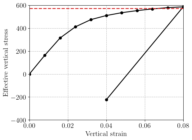
Below, we plot the evolution of the effective vertical stress as a function of the imposed loading. One can observe an initial elastic phase followed by a strongly non-linear hardening phase. Note the effective stress seems to approach the value in red given by \(\dfrac{2}{\sqrt{3}}\sigma_u(1-2R/W) f\) where \(f\approx 2\ln(2)\) which is an upper-bound estimate of the plate collapse load. As expected for plasticity problems, the unloading stage is indeed elastic and exhibits residual stresses.
plt.figure()
plt.plot(Eps * t_list, Sig, "-ok")
plt.axhline(1 / np.sqrt(3) * sigu.value * 2*np.log(2), color="C3", linestyle="--")
plt.xlabel("Vertical strain")
plt.ylabel(r"Effective vertical stress")
plt.show()
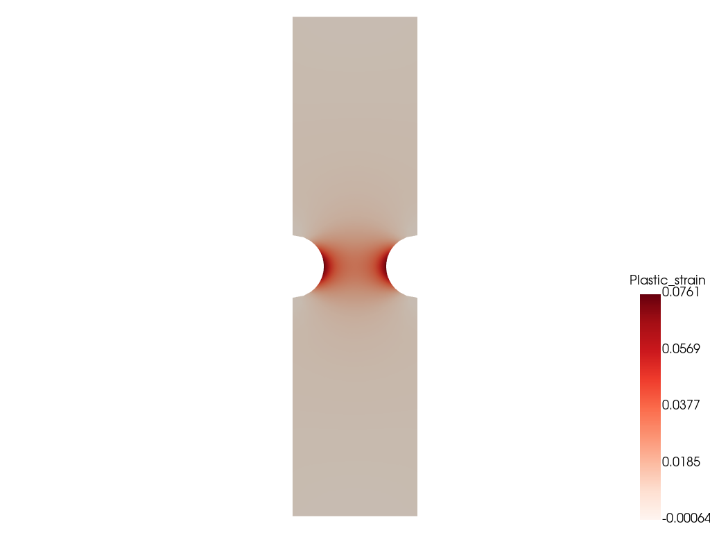
We can also plot the distribution of equivalent plastic strain \(p\) at the final stage using pyvista. One can clearly observe the formation of plastic hinges near the clamped supports and a more diffuse plastic field at the beam mid-span.
import pyvista
from dolfinx import plot

topology, cell_types, geometry = plot.vtk_mesh(Vp)
grid = pyvista.UnstructuredGrid(topology, cell_types, geometry)
grid.point_data["Plastic_strain"] = p.x.array
grid.set_active_scalars("Plastic_strain")
pl = pyvista.Plotter()
pl.add_mesh(grid, cmap="Reds", scalar_bar_args={"vertical": True})
pl.view_xy()
pl.show()
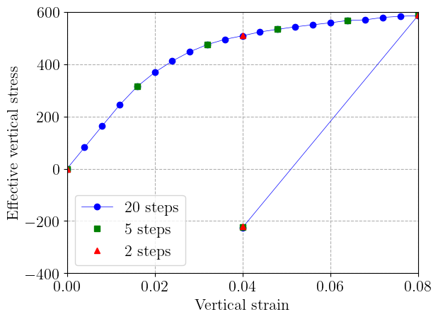
We can also check that this incremental formulation is not very sensitive to the number of increments in a monotonic loading process.
plt.figure()
for l, style in zip([20, 5, 2], ["-ob", "sg", "^r"]):
    X = np.loadtxt(f"elastoplasticity_{l}steps.csv", skiprows=1, delimiter=",")
    plt.plot(X[:, 0], X[:, 1], style, linewidth=0.5, label=f"{l} steps")
plt.xlabel("Vertical strain")
plt.ylabel("Effective vertical stress")
plt.legend()
plt.show()
References#
Bernard Halphen and Quoc Son Nguyen. Sur les matériaux standard généralisés. Journal de mécanique, 14(1):39–63, 1975.
Michael Ortiz and Laurent Stainier. The variational formulation of viscoplastic constitutive updates. Computer methods in applied mechanics and engineering, 171(3-4):419–444, 1999.