Computing the Hosford plane stress yield surface

This short demo shows how to define a perfectly plastic material associated with the Hosford equivalent stress and how to compute its yield surface in plane stress conditions.\(\newcommand{\bsig}{\boldsymbol{\sigma}}\newcommand{\beps}{\boldsymbol{\varepsilon}}\)

See also

This demo is inspired by the MFront Hosford tutorial.

The Hosford yield surface is defined by:

\[ f(\bsig) = \sigma_\text{eq}^\text{H} - \sigma_0 = \left(\dfrac{1}{2}\left(|\sigma_I-\sigma_{II}|^a+|\sigma_I-\sigma_{III}|^a+|\sigma_{II}-\sigma_{III}|^a\right)\right)^{1/a} - \sigma_0 \]

where \(\sigma_\text{eq}^\text{H}\) is the Hosford equivalent stress associated with the shape parameter \(a\). For \(a=2\), this reduces to the von Mises norm and, for \(a\to\infty\), we obtain the Tresca norm.

We first define a GeneralIsotropicHardening JAX material without any hardening.

import numpy as np
import matplotlib.pyplot as plt
from dolfinx_materials.jax_materials import (
    GeneralIsotropicHardening,
    LinearElasticIsotropic,
    Hosford_stress,
)
import jax

plt.ioff()

E = 70e3
nu = 0.3
elastic_model = LinearElasticIsotropic(E, nu)


a = 10.0
sig0 = 500.0
material = GeneralIsotropicHardening(
    elastic_model, lambda sig: sig0, lambda sig: Hosford_stress(sig, a=a)
)

An NVIDIA GPU may be present on this machine, but a CUDA-enabled jaxlib is not installed. Falling back to cpu.

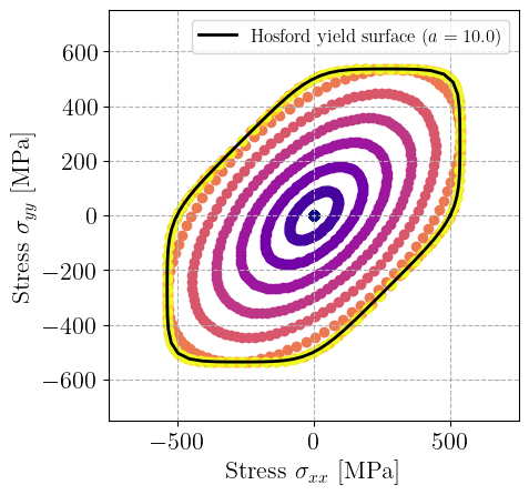
We want to plot the corresponding yield surface in the plane stress domain \((\sigma_{xx}, \sigma_{yy}, \sigma_{zz}=0)\). We generate Nbatch strain loading directions in the \((\varepsilon_{xx},\varepsilon_{yy})\) plane and we will increment the strain proportionally up to a maximum value \(\varepsilon_{max}=10^{-2}\).

eps = 1e-2
Nbatch = 100
theta = np.linspace(0, 2 * np.pi, Nbatch)
Eps = np.vstack(
    [np.array([eps * np.cos(t), eps * np.sin(t), 0, 0, 0, 0]) for t in theta]
)
material.set_data_manager(Eps.shape[0])
state = material.get_initial_state_dict()

Since the constitutive equation is strain-driven, we need to adjust the out-of-plane strain \(\varepsilon_{zz}\) to satisfy the plane stress condition \(\sigma_{zz}=0\). To do so, we will apply an additional Newton method after each computation to enforce \(\sigma_{zz}=0\). This Newton step amounts to find the out-of-plane strain correction \(\delta\varepsilon_{zz}\) such that:

\[ \sigma_{zz}(\beps+\delta\varepsilon_{zz}e_z\otimes e_z) \approx \sigma_{zz}(\beps) + \dfrac{\partial \sigma_{zz}}{\partial \varepsilon_{zz}}\delta\varepsilon_{zz} = 0 \]

Hence, the Newton correction step involves the out-of-plane component \(\mathbb{C}^\text{tang}_{zzzz}\) of the tangent operator and reads:

\[ \delta\varepsilon_{zz} = -\sigma_{zz}(\beps)/\mathbb{C}^\text{tang}_{zzzz} \]

We benefit from JAX automatic vectorization by writing this correction step for a single load case and use jax.vmap to loop overall loading paths automatically.

def correct_epszz(eps, sig, Ct):
    return (-sig[2]) / Ct[2, 2]


global_correct = jax.vmap(jax.jit(correct_epszz))

The tolerance of this plane stress correction will be measured by the out-of-plane stress residual \(|\sigma_{zz}/E|\). We define a tolerance tol=1e-6 and a maximum number of iterations. We then loop over each load step increment, compute the stress for \(\varepsilon_{zz}=0\) and then do the plane stress correction until converging. Finally, we plot the resulting distribution of stresses and compare against the analytical equation of the Hosford yield surface.

tol = 1e-6
niter_max = 20
depszz = np.zeros((Nbatch,))
times = np.linspace(0, 1.0, 10)
cmap = plt.get_cmap("plasma")
colors = cmap(times / max(times))
fig, ax = plt.subplots()
for i, t in enumerate(times):
    print(f"Increment {i+1}/{len(times)}")
    Eps_i = t * Eps
    res_plane = np.ones((Nbatch,))
    k = 0
    while np.any(res_plane > tol) and k < niter_max:
        sig, isv, Ct = material.integrate(Eps_i)
        depszz = global_correct(Eps_i, sig, Ct)
        Eps_i[:, 2] += depszz
        res_plane = np.abs(sig[:, 2] / E)
        k += 1
    if k >= niter_max:
        raise ValueError("Maximum number of iterations reached.")

    material.data_manager.update()
    ax.scatter(sig[:, 0], sig[:, 1], color=colors[i])


def normalize_by_Hosford(sig):
    sig_eq = Hosford_stress(sig)
    return sig * sig0 / sig_eq


sig_list = np.vstack([np.array([np.cos(t), np.sin(t), 0, 0, 0, 0]) for t in theta])
Sig = jax.vmap(normalize_by_Hosford)(sig_list)

ax.plot(Sig[:, 0], Sig[:, 1], "-k", label=rf"Hosford yield surface $(a={a})$")
ax.set_xlabel(r"Stress $\sigma_{xx}$ [MPa]")
ax.set_ylabel(r"Stress $\sigma_{yy}$ [MPa]")
ax.legend(fontsize=12)
ax.set_xlim(-1.5 * sig0, 1.5 * sig0)
ax.set_ylim(-1.5 * sig0, 1.5 * sig0)
ax.set_aspect("equal")
plt.show()

Increment 1/10

Increment 2/10
Increment 3/10
Increment 4/10
Increment 5/10
Increment 6/10
Increment 7/10
Increment 8/10
Increment 9/10
Increment 10/10