Finite-element simulations of JAX elastoplasticity

In this example, we show how to use an elastoplastic JAXMaterial within a FEniCSx finite-element simulation. We use a von Mises elastoplastic material with a general isotropic hardening model. The JAX implementation of such a behavior is described in .

We start by loading the relevant modules. In particular, we will make use of the QuadratureMap object available in dolfinx_materials.quadrature_map which handles the exchange of information between FEniCSx and custom material objects, here a JAXMaterial.

import numpy as np
import matplotlib.pyplot as plt
import jax.numpy as jnp
from mpi4py import MPI
import ufl
from dolfinx import io, fem
from dolfinx.cpp.nls.petsc import NewtonSolver
from dolfinx.common import list_timings, TimingType
from dolfinx_materials.quadrature_map import QuadratureMap
from dolfinx_materials.solvers import NonlinearMaterialProblem
from dolfinx_materials.jax_materials import (
    vonMisesIsotropicHardening,
    LinearElasticIsotropic,
)
from generate_mesh import generate_perforated_plate

An NVIDIA GPU may be present on this machine, but a CUDA-enabled jaxlib is not installed. Falling back to cpu.

Material definition

We first define our elastoplastic material using the ElastoPlasticIsotropicHardening class which represents a JAX von Mises elastoplastic material which takes as input arguments a JAX LinearElasticIsotropic material and a custom hardening yield stress function. Here we use a Voce-type exponential harding such that:

\[ \sigma_Y(p) = \sigma_0 + (\sigma_u-\sigma_0)\exp(-bp) \]

where \(\sigma_0\) and \(\sigma_u\) are the initial and final yield stresses respectively and \(b\) is a hardening parameter controlling the rate of convergence from \(\sigma_0\) to \(\sigma_u\) as a function of the cumulated plastic strain \(p\).

E = 70e3
sig0 = 350.0
sigu = 500.0
b = 1e3
elastic_model = LinearElasticIsotropic(E=70e3, nu=0.3)


def yield_stress(p):
    return sig0 + (sigu - sig0) * (1 - jnp.exp(-b * p))


material = vonMisesIsotropicHardening(elastic_model, yield_stress)

Problem setup

We then generate the mesh of a rectangular plate of dimensions \(L_x\times L_y\) perforated by a circular hole of radius R at its center using gmsh. mesh_sizes=(fine_size, coarse_size) enables to locally refine the mesh size near the hole. The bottom and top faces of the plate are tagged 1 and 2 respectively.

Lx = 1.0
Ly = 2.0
R = 0.2
mesh_sizes = (0.008, 0.2)
domain, markers, facets = generate_perforated_plate(Lx, Ly, R, mesh_sizes)
ds = ufl.Measure("ds", subdomain_data=facets)

We define the function space for the displacement \(\boldsymbol{u}\), interpolated here with quadratic Lagrange elements. We apply prescribed Dirichlet boundary conditions on the bottom and top dofs. For the consitutive equation, we use a quadrature degree equal to twice the degree of the associated strain i.e. 2*(order-1)=2 here.

order = 2
deg_quad = 2 * (order - 1)
shape = (2,)

V = fem.functionspace(domain, ("P", order, shape))
bottom_dofs = fem.locate_dofs_topological(V, 1, facets.find(1))
top_dofs = fem.locate_dofs_topological(V, 1, facets.find(2))

uD_b = fem.Function(V)
uD_t = fem.Function(V)
bcs = [fem.dirichletbc(uD_t, top_dofs), fem.dirichletbc(uD_b, bottom_dofs)]

Now, we define the QuadratureMap object associated with the elastoplastic material. We check that the material has only one gradient field, here the field "Strain" and one flux field, here the field "Stress". We register the UFL object strain(u) corresponding to the vectorial Mandel representation of the strain components.

def strain(u):
    return ufl.as_vector(
        [
            u[0].dx(0),
            u[1].dx(1),
            0.0,
            1 / np.sqrt(2) * (u[1].dx(0) + u[0].dx(1)),
            0.0,
            0.0,
        ]
    )

u = fem.Function(V)

qmap = QuadratureMap(domain, deg_quad, material)
print("Gradients", material.gradient_names)
print("Fluxes", material.flux_names)
qmap.register_gradient(material.gradient_names[0], strain(u))

Gradients ['Strain']
Fluxes ['Stress']

We can then use the abstract flux field "Stress" to define the weak formulation in small strain conditions and use qmap.derivative to define the associated tangent form using AutoDiff.

du = ufl.TrialFunction(V)
v = ufl.TestFunction(V)

sig = qmap.fluxes["Stress"]
Res = ufl.dot(sig, strain(v)) * qmap.dx
Jac = qmap.derivative(Res, u, du)

Next, the custom nonlinear problem is defined with the class NonlinearMaterialProblem as well as the corresponding Newton solver.

problem = NonlinearMaterialProblem(qmap, Res, Jac, u, bcs)
newton = NewtonSolver(MPI.COMM_WORLD)
newton.rtol = 1e-6
newton.atol = 1e-6
newton.convergence_criterion = "residual"
newton.max_it = 20

We then loop over a set of imposed vertical strains, apply the corresponding imposed displacement boundary condition on the top surface, solve the problem and then compute plastic and stress fields projected onto a DG space for visualization. Finally, we use the imposed displacement field to compute the associated resultant force in a consistent manner, see for more details.

out_file = "elastoplasticity.pvd"
vtk = io.VTKFile(domain.comm, out_file, "w")

N = 15
Eyy = np.linspace(0, 10e-3, N + 1)
Force = np.zeros_like(Eyy)
nit = np.zeros_like(Eyy)
for i, eyy in enumerate(Eyy[1:]):
    u_imp = eyy*Ly
    uD_t.vector.array[1::2] = u_imp

    converged, it = problem.solve(newton, print_solution=False)

    p = qmap.project_on("p", ("DG", 0))
    stress = qmap.project_on("Stress", ("DG", 0))

    Force[i + 1] = fem.assemble_scalar(fem.form(ufl.action(Res, u))) / u_imp

    syy = stress.sub(1).collapse()
    syy.name = "Stress"
    vtk.write_function(u, i + 1)
    vtk.write_function(p, i + 1)
    vtk.write_function(syy, i + 1)
    nit[i+1] = it

vtk.close()

Results

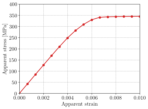
We plot the evolution of the apparent vertical stress as a function of the imposed apparent strain. We observe a progressive onset of plasticity after a first elastic phase. The apparent stress then saturates, reaching a perfectly plastic plateau associated with plastic collapse of the plate.

plt.plot(Eyy, Force/Lx, "-oC3")
plt.xlabel("Apparent strain")
plt.ylabel("Apparent stress [MPa]")
plt.ylim(0, 400)
plt.show()

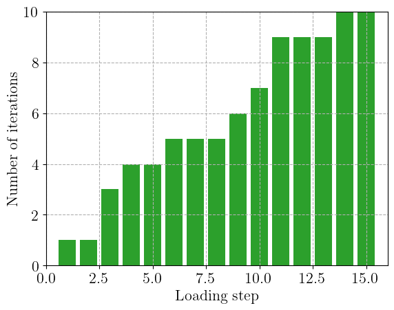
We report below the evolution of the number of Newton iterations for each load step. We can see that in the first iterations, convergence is reached in 1 iteration only, corresponding to the elastic stage. The number of iterations then increases, the final stages corresponding to the plastic collapse needing around 10 iterations to converge.

plt.bar(np.arange(N + 1), nit, color="C2")
plt.xlabel("Loading step")
plt.ylabel("Number of iterations")
plt.xlim(0, N+1)
plt.show()

We list the total timings. We can check that the constitutive update represents only a small fraction of the total computing time which is mostly dominated by the cost of solving the global linear system at each global Newton iteration.

from dolfinx.common import timing
constitutive_update_time = timing("Constitutive update")[2]
linear_solve_time = timing("PETSc Krylov solver")[2]
print(f"Total time spent in constitutive update {constitutive_update_time:.2f}s")
print(f"Total time spent in global linear solver {linear_solve_time:.2f}s")

Total time spent in constitutive update 4.64s
Total time spent in global linear solver 39.09s