Transient heat equation with phase change#
\(\newcommand{\bj}{\mathbf{j}} \renewcommand{\div}{\operatorname{div}}\) In this demo, we expand on the stationary nonlinear heat transfer demo and consider a transient heat equation with non-linear heat transfer law including solid/liquid phase change. This demo corresponds to the TTNL02 elementary test case of the Code_Aster finite-element software.
Transient heat equation using an enthalpy formulation#
The transient heat equation writes:
where \(\rho\) is the material density, \(C_p\) the heat capacity (at constant pressure) per unit of mass, \(r\) represents heat sources and \(\bj\) is the heat flux.
In the case of phase changes, the heat capacity exhibits large discontinuities near the transition temperature. It is therefore more suitable to work with the enthalpy density defined as:
yielding the following heat equation:
Description of the non-linear heat transfer law with phase change#
The thermal material is described by the following non linear Fourier Law:
where the thermal conductivity \(k\) is initially assumed to be given by:
where \(k_s\) (resp. \(k_l\)) denotes the solid (resp. liquid) phase conductivity and \(T_m\) is the solid/liquid transition temperature.
The enthalpy is assumed to be given by:
where \(c_s=\rho_sC_{p,s}\) (resp. \(c_l=\rho_lC_{p,l}\)) is the volumetric heat capacity of the solid (resp. liquid) phase. It can be observed that the enthalpy exhibits a discontinuity at the phase transition equal to \(\Delta h_{s/l}\) which represents the latent heat of fusion per unit volume.

A smoothed version#
The enthalpy discontinuity \(\Delta h_{s/l}\) poses convergence difficulties for the Newton resolution. A classical remedy consists in considering a smoothed version of the previous law, such as:
and
where \(T_{smooth}=T_l-T_s\) is a small transition temperature interval between \(T_s=T_m-T_\text{smooth}/2\) the solidus temperature and \(T_l=T_m+T_\text{smooth}/2\) the liquidus temperature.
MFront implementation#
Gradient, flux and tangent operator blocks#
Similarly to the stationary nonlinear heat transfer demo, the MFront implementation relies on the DefaultGenericBehaviour DSL and declares the pair of temperature gradient and heat flux. In addition, the volumic enthalpy \(h\) is also declared as an internal state variable. In addition to the two tangent operator blocks ∂j∕∂Δ∇T and ∂j∕∂ΔT already discussed in the first demo, we also declare the additional block ∂h∕∂ΔT, referring to the fact that the enthalpy will vary with the temperature and will enter the transient heat equation.
@DSL DefaultGenericBehaviour;
@Behaviour HeatTransferPhaseChange;
@Author Thomas Helfer / Jérémy Bleyer;
@Date 15 / 02 / 2019;

@Gradient TemperatureGradient ∇T;
∇T.setGlossaryName("TemperatureGradient");

@Flux HeatFlux j;
j.setGlossaryName("HeatFlux");

@StateVariable real h;
h.setEntryName("Enthalpy"); //per unit of volume

@AdditionalTangentOperatorBlock ∂j∕∂ΔT;
@AdditionalTangentOperatorBlock ∂h∕∂ΔT;
Material parameters and local variables#
We now declare the various material properties corresponding to those of aluminum. The material parameters are assumed to be uniform for both phases. Finally, we also introduce the smoothing temperature width \(T_\text{smooth}\).
@Parameter Tₘ = 933.15;        // [K]
Tₘ.setEntryName("MeltingTemperature");
@Parameter kₛ = 210;           // [W/m/K]
kₛ.setEntryName("SolidConductivity");
@Parameter cₛ = 3.e6;          // [J/m^3/K]
cₛ.setEntryName("SolidHeatCapacity");
@Parameter kₗ = 95;            // [W/m/K]
kₗ.setEntryName("LiquidConductivity");
@Parameter cₗ = 2.58e6;        // [J/m^3/K]
cₗ.setEntryName("LiquidHeatCapacity");
@Parameter Δhₛₗ = 1.08048e9;   // [J/m^3]
Δhₛₗ.setEntryName("FusionEnthalpy");
@Parameter Tₛₘₒₒₜₕ = 0.1;      // smoothing temperature width [K]
Tₛₘₒₒₜₕ.setEntryName("Tsmooth");
We define some local variables corresponding to the values of the conductivity \(k\), the volumetric heat capacity \(c\) and the derivative of the heat conductivity with respect to the temperature.
@LocalVariable thermalconductivity k;
@LocalVariable real c;
@LocalVariable real ∂k∕∂T;
Integration of the behaviour#
Again, the behaviour integration is straightforward: after computing the temperature at the end of the time step T_, we compute the thermal
conductivity, its derivative with respect to the temperature, the volumetric enthalpy and the volumetric heat capacity depending on whether T_ belongs to the solid state (\(T\leq T_s\)), the liquid state (\(T\geq T_l\)) or to the transition region (\(T_s \leq T \leq T_l\)). We finish by computing the heat flux.
@Integrator {
  const auto T_ = T + ΔT;     // current temperature
  const auto Tₛ = Tₘ-Tₛₘₒₒₜₕ/2; // solidus temperature
  const auto Tₗ = Tₘ+Tₛₘₒₒₜₕ/2; // liquidus temperature
  if(T_<Tₛ){                  // solid state
    k = kₛ;
    c = cₛ;
    h = cₛ*T_;
    ∂k∕∂T = 0.;
  } else if (T_ > Tₗ) {        // liquid state
    k = kₗ;
    c = cₗ;
    h = cₗ*(T_-Tₗ)+Δhₛₗ+cₛ*Tₛ+(cₛ+cₗ)*Tₛₘₒₒₜₕ/2;
    ∂k∕∂T = 0.;
  } else {                    // solid/liquid smooth transition
    k = kₛ + (kₗ-kₛ)*(T_-Tₛ)/Tₛₘₒₒₜₕ;
    h = cₛ*Tₛ+((cₛ+cₗ)/2+Δhₛₗ/Tₛₘₒₒₜₕ)*(T_-Tₛ);
    c = Δhₛₗ/(Tₗ-Tₛ);
    ∂k∕∂T = -(kₗ-kₛ)/Tₛₘₒₒₜₕ;
  }
  // heat flux
  j = -k ⋅ (∇T + Δ∇T);
}  // end of @Integrator
Tangent operator#
The computation of the tangent operator blocks is then straightforward:
@TangentOperator {
  ∂j∕∂Δ∇T = -k * tmatrix<N, N, real>::Id();
  ∂j∕∂ΔT = ∂k∕∂T * (∇T + Δ∇T);
  ∂h∕∂ΔT = c;
}  // end of @TangentOperator
FEniCSx implementation#
Geometry and material#
We consider a rectanglar domain of length 0.1 with imposed temperatures T0 (resp. Ti) on the left (resp. right) boundaries. We look here for the temperature field T using a \(P^2\)-interpolation which is initially at the uniform temperature Ti.
import numpy as np
import matplotlib.pyplot as plt
import ufl
import os
from mpi4py import MPI
from dolfinx import fem, mesh
from dolfinx_materials.quadrature_map import QuadratureMap
from dolfinx_materials.solvers import NonlinearMaterialProblem
from dolfinx_materials.mfront import MFrontMaterial

current_path = os.getcwd()

length = 0.1
width = 0.01
Nx = 1000
Ny = 1
domain = mesh.create_rectangle(
    MPI.COMM_WORLD,
    [(0, 0), (length, width)],
    [Nx, Ny],
    cell_type=mesh.CellType.quadrilateral,
)

V = fem.functionspace(domain, ("P", 2))
T = fem.Function(V, name="Temperature")


def left(x):
    return np.isclose(x[0], 0.0)


def right(x):
    return np.isclose(x[0], length)


def bottom(x):
    return np.isclose(x[1], 0.0)


Tl = 853.15
Tr = 1013.15
T.x.petsc_vec.set(Tr)

left_dofs = fem.locate_dofs_geometrical(V, left)
right_dofs = fem.locate_dofs_geometrical(V, right)
bottom_dofs = fem.locate_dofs_geometrical(V, bottom)  # used for postprocessing

bcs = [fem.dirichletbc(Tl, left_dofs, V), fem.dirichletbc(Tr, right_dofs, V)]
We now load the material behaviour HeatTransferPhaseChange and also change the default value of Tsmooth to a slightly larger one (but still sufficiently small). Note that the mesh must be sufficiently refined to use a smaller value. Indeed, the spatial resolution must be able to capture with a few elements the sharp transition which will occur during the phase change. We also verify that 3 different tangent blocks have indeed been defined, the last one involving the internal state variable Enthalpy with respect to the temperature.
material = MFrontMaterial(
    os.path.join(current_path, "src/libBehaviour.so"),
    "HeatTransferPhaseChange",
    hypothesis="plane_strain",
    parameters={"Tsmooth": 1.0},
)
print(["d{}_d{}".format(*t) for t in material.tangent_blocks])
['dHeatFlux_dTemperatureGradient', 'dHeatFlux_dTemperature', 'dEnthalpy_dTemperature']
Time discretization of the heat equation#
The heat equation must also be discretized in time. We use here the \(\theta\)-method and approximate:
where \(\star_{t=t_{n+\theta}}= \theta\star_{t=t_{n+1}}+(1-\theta)\star_{t=t_{n}}\).
The weak formulation therefore reads (in the absence of source terms): Find \(T\in V\) such that:
in which, at time \(t_{n+1}\), both the enthalpy \(h_{t=t_{n+1}}\) and the heat flux \(\mathbf{j}_{t=t_{n+1}}\) are non-linear functions of the unknown temperature.
Problem formulation#
To write the above non-linear time-dependent weak formulation, we first need to register to the QuadratureMap object the corresponding gradient and external state variable. Then we can get the heat flux j (as a flux) and the enthalpy h (as an internal state variable).
Note that without explicitly calling the behaviour law or setting its value, the enthalpy function h will be initially of value 0. To initialize its value, we write qmap.update() which calls the behaviour integration and updates the internal state variable and flux values.
To implement the \(\theta\) time discretization scheme, we will also need to keep track of the enthalpy and heat flux values at the previous time step. We can simply define these new functions as copies of h and j. Doing so, h_old and j_old will also be Quadrature functions.
We then compute the corresponding jacobian form with qmap.derivative.
T_ = ufl.TestFunction(V)
dT = ufl.TrialFunction(V)

qmap = QuadratureMap(domain, 2, material)
qmap.register_gradient("TemperatureGradient", ufl.grad(T))
qmap.register_external_state_variable("Temperature", T)

j = qmap.fluxes["HeatFlux"]
h = qmap.internal_state_variables["Enthalpy"]

qmap.update()  # call a first time the behaviour law to update the value of the internal state variables

j_old = j.copy()
h_old = h.copy()


dt = fem.Constant(domain, 0.0)
theta = fem.Constant(domain, 1.0)

j_theta = theta * j + (1 - theta) * j_old

Res = (T_ * (h - h_old) - dt * ufl.dot(ufl.grad(T_), j_theta)) * qmap.dx
Jac = qmap.derivative(Res, T, dT)
We then set up the corresponding nonlinear problem and solver options.
petsc_options = {
    "snes_type": "newtonls",
    "snes_linesearch_type": "none",
    "snes_atol": 1e-6,
    "snes_rtol": 1e-6,
    "ksp_type": "preonly",
    "pc_type": "lu",
    "pc_factor_mat_solver_type": "mumps",
}
problem = NonlinearMaterialProblem(
    qmap,
    Res,
    T,
    bcs=bcs,
    J=Jac,
    petsc_options_prefix="phase_change",
    petsc_options=petsc_options,
)
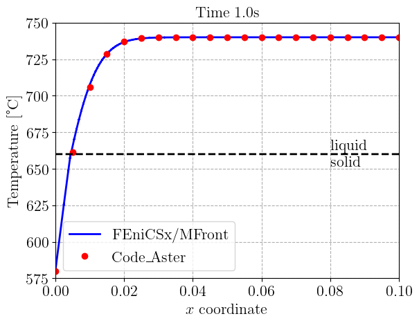
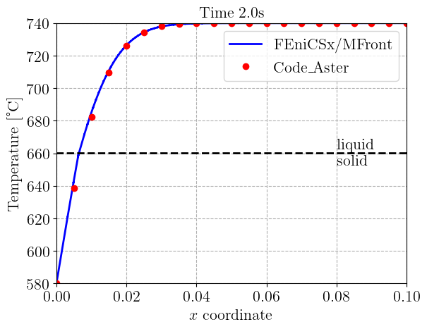
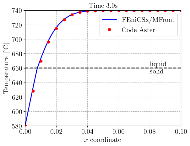
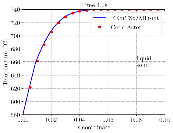
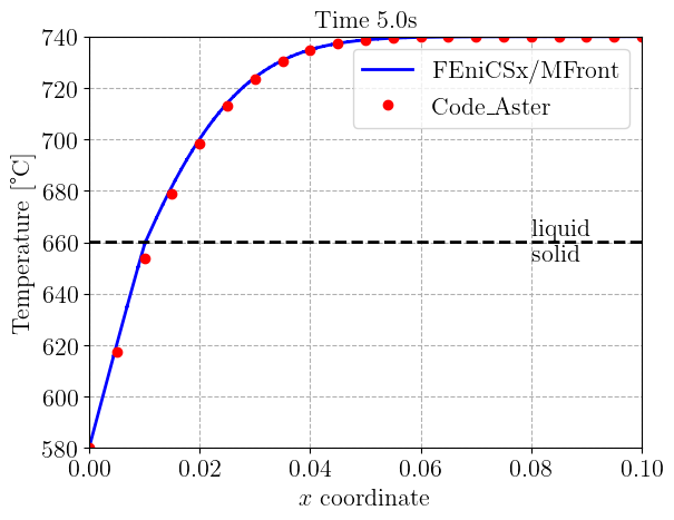
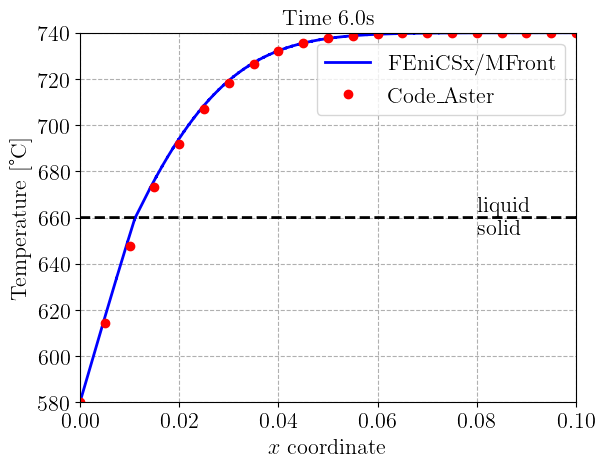
Time-stepping loop and comparison with code_Aster results#
We now implement the time-stepping loop which simply solves the non-linear problem and update the fields corresponding to the values at the previous time step. We also load the values of the one-dimensional temperature field \(T(x, t)\) given in the code_Aster test-case and compare them with what we obtain every second.
cA_results = np.loadtxt(
    os.path.join(current_path, "results_code_Aster.csv"), delimiter=","
)
code_Aster_times = np.arange(1, 7)
Nsteps = 60
times = np.linspace(0, 6.0, Nsteps + 1)
x = V.tabulate_dof_coordinates()[bottom_dofs, 0]  # x position of dofs
for t, delta_t in zip(times[1:], np.diff(times)):
    dt.value = delta_t

    problem.solve()
    converged = problem.solver.getConvergedReason()
    num_iter = problem.solver.getIterationNumber()
    assert converged

    fem.petsc.assign(h.x.petsc_vec, h_old)  # update enthalpy
    fem.petsc.assign(j.x.petsc_vec, j_old)  # update heat flux

    sol_time = np.isclose(t, code_Aster_times)
    if any(sol_time):
        plt.figure()
        plt.title("Time {:0.1f}s".format(t), fontsize=16)
        ax1 = plt.gca()
        ax1.set_xlabel("$x$ coordinate")
        ax1.set_ylabel("Temperature [°C]")
        T_val = T.x.array[bottom_dofs]
        ax1.plot(
            x,
            T_val - 273.15,
            "-b",
            label="FEniCSx/MFront",
        )
        ax1.plot(
            cA_results[:, 0],
            cA_results[:, np.where(sol_time)[0] + 1],
            "or",
            label="Code\_Aster",
        )
        Tm = material.get_parameter("MeltingTemperature") - 273.15
        ax1.plot(x, Tm + 0 * x, "--k")
        ax1.annotate("liquid\nsolid", xy=(0.08, Tm), fontsize=16, va="center")
        plt.legend()
        plt.show()