Hyperelastic heterogeneous material

Hyperelastic heterogeneous material#

In this demo, we show how to define a problem containing a call to a MFront behavior on a subset of cells while defining the behavior on the remaining part of the domain using UFL.

Tip

This demo also works in parallel.

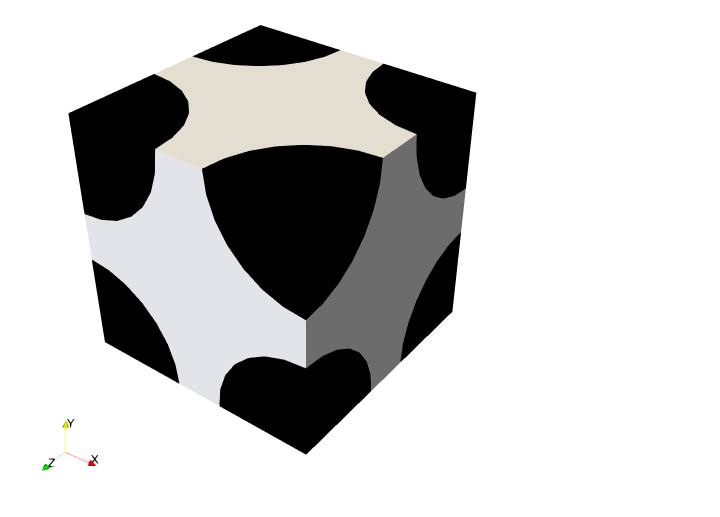
We consider a unit square consisting of circular inclusions of radius \(R=0.4\) located at the 8 vertices of the unit cube. The matrix domain \(\Omega_\text{m}\) (tagged 1) consists of a Ogden hyperelastic material implemented with MFront. The inclusions domain \(\Omega_\text{i}\) (tagged 2) is assumed to be much stiffer and will be described by a Saint-Venant Kirchhoff (SVK) material of modulus \(E_\text{pen} = 10^3\) GPa and Poisson ratio \(\nu=0\). This behavior will be implemented in pure UFL.

Meshing#

We start by importing the relevant modules and defining the geometrical characteristics.

import numpy as np
from mpi4py import MPI
import gmsh
import ufl
from petsc4py import PETSc
from dolfinx import fem, io
from dolfinx.cpp.nls.petsc import NewtonSolver
from dolfinx_materials.quadrature_map import QuadratureMap
from dolfinx_materials.material.mfront import MFrontMaterial
from dolfinx_materials.solvers import NonlinearMaterialProblem
from dolfinx_materials.utils import (
    symmetric_tensor_to_vector,
    nonsymmetric_tensor_to_vector,
)

comm = MPI.COMM_WORLD
rank = comm.rank

dim = 3
L = 1.0
R = 0.4
hsize = 0.1

centers = np.array(
    [
        [0.0, 0.0, 0.0],
        [L, 0.0, 0.0],
        [0.0, L, 0.0],
        [0.0, 0.0, L],
        [L, L, 0.0],
        [L, 0.0, L],
        [0.0, L, L],
        [L, L, L],
    ]
)

We then define the mesh using gmsh.

Problem position#

Next, we define fixed displacement boundary conditions on the left boundary and will impose a uniform horizontal displacement on the right surface. For this problem, we use \(\mathbb{P}_2\) Lagrange elements and a quadrature rule degree of 2.

fdim = dim - 1
domain.topology.create_connectivity(fdim, dim)

order = 2
V = fem.functionspace(domain, ("P", order, (3,)))
deg_quad = 2 * (order-1)

left_dofs = fem.locate_dofs_topological(V, fdim, facets.find(1))
right_dofs = fem.locate_dofs_topological(V, fdim, facets.find(2))


uD = fem.Constant(domain, np.zeros((dim,)))
bcs = [
    fem.dirichletbc(np.zeros((dim,)), left_dofs, V),
    fem.dirichletbc(uD, right_dofs, V),
]

The weak form writes in the present case as follows:

\[ \newcommand{\be}{\boldsymbol{e}} \newcommand{\bu}{\boldsymbol{u}} \newcommand{\bv}{\boldsymbol{v}} \newcommand{\dOm}{\,\text{d}\Omega} \int_{\Omega_\text{m}}\boldsymbol{P}(\bu):\nabla\bv \dOm + \int_{\Omega_\text{i}}\boldsymbol{S}(\bu):\delta\be_\text{GL}(\bu;\bv) \dOm = 0 \quad \forall\bv\in V \]

where \(\boldsymbol{P}(\bu)\) denotes the matrix first Piola-Kirchhoff stress obtained from the MFront Ogden material, \(\boldsymbol{S}(\bu) = E_\text{pen}\be_\text{GL}(\bu)\) denotes the second Piola-Kirchhoff stress associated with the quasi-rigid SVK material, \(\be_\text{GL}(\bu)\) is the Green-Lagrange strain and \(\delta\be_\text{GL}(\bu;\bv)\) its variation in direction \(\bv\).

We define below helper functions for implementing the weak form. Note that we use the symmetric_tensor_to_vector and nonsymmetric_tensor_to_vector functions from dolfinx_material.utils to convert tensors to vectorial representation following Conventions for representing tensors. We first implement the inclusions contribution to the total residual weak form using pure UFL.

Id = ufl.Identity(dim)


def GL_strain(u):
    F = Id + ufl.grad(u)
    eGL = (F.T*F - Id)/2
    return symmetric_tensor_to_vector(eGL)


def dGL_strain(u, v):
    return ufl.derivative(GL_strain(u), u, v)


def F(u):
    return nonsymmetric_tensor_to_vector(Id + ufl.grad(u))


def dF(u, v):
    return ufl.derivative(F(u), u, v)

du = ufl.TrialFunction(V)
v = ufl.TestFunction(V)
u = fem.Function(V, name="Displacement")

dx = ufl.dx(subdomain_data=subdomains)

E_pen = fem.Constant(domain, 1e12)
Res_inclusions = ufl.dot(E_pen * GL_strain(u), dGL_strain(u, v)) * dx(2)

Second, we define the Ogden MFrontMaterial instance and implement the matrix contribution to the weak form residual. Note that we enforce cells=cells_matrix, asking the QuadratureMap to call the constitutive update only at quadrature points located within these matrix cells.

material = MFrontMaterial(
    "src/libBehaviour.so",
    "Ogden",
)

cells_matrix = subdomains.find(1)
qmap = QuadratureMap(domain, deg_quad, material, cells=cells_matrix)
qmap.register_gradient("DeformationGradient", F(u))
qmap.dx = qmap.dx(subdomain_data=subdomains)

PK1 = qmap.fluxes["FirstPiolaKirchhoffStress"]
Res_matrix = ufl.dot(PK1, dF(u, v)) * dx(1)

Finally, the total residual is the sum of both residuals. We also include a normalizing factor since all stress quantities are expressed in Pa units.

normalization_factor = fem.Constant(domain, 1e-6)
Res = normalization_factor * (Res_matrix + Res_inclusions)
Jac = qmap.derivative(Res, u, du)

Resolution#

Next, we define the custom nonlinear problem, the corresponding Newton solver and the PETSc Krylov solver used to solve the linear systems within Newton’s method. We use here a GMRES iterative solver preconditioned with a Geometric Algebraic MultiGrid preconditioner.

problem = NonlinearMaterialProblem(qmap, Res, Jac, u, bcs)

newton = NewtonSolver(comm)
newton.rtol = 1e-6
newton.atol = 1e-6
newton.convergence_criterion = "residual"

# Set solver options
ksp = newton.krylov_solver
opts = PETSc.Options()
option_prefix = ksp.getOptionsPrefix()
opts[f"{option_prefix}ksp_type"] = "gmres"
opts[f"{option_prefix}ksp_rtol"] = 1e-8
opts[f"{option_prefix}pc_type"] = "gamg"
ksp.setFromOptions()

file_results = io.VTKFile(
    domain.comm,
    f"{material.name}_results.pvd",
    "w",
)

N = 10
Exx = np.linspace(0, 20e-2, N + 1)

file_results.write_function(u, 0)
for i, exx in enumerate(Exx[1:]):
    uD.value[0] = exx*L

    if rank == 0:
        print(f"Increment {i}")

    converged, it = problem.solve(newton)

    file_results.write_function(u, i+1)


file_results.close()

Timings#

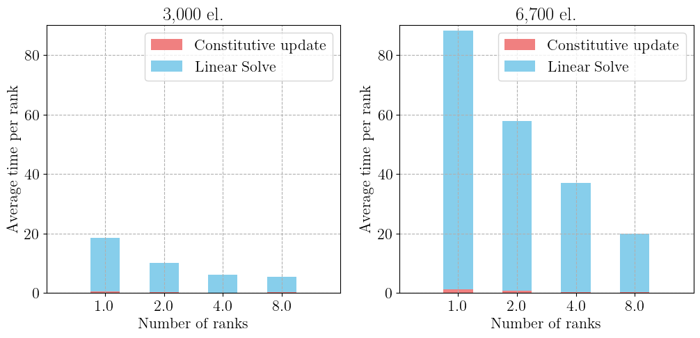
We list the total timings by gathering all times spent on each rank and compute the average per rank. We can check that the constitutive update represents only a small fraction of the total computing time which is mostly dominated by the cost of solving the global linear system at each global Newton iteration.

from dolfinx.common import timing

constitutive_update_time = timing("Constitutive update")[2]
linear_solve_time = timing("PETSc Krylov solver")[2]

# Gather all times on rank 0
all_times = None
if rank == 0:
    all_times = np.zeros((comm.size, 2))
comm.Gather(np.array([constitutive_update_time, linear_solve_time]), all_times, root=0)

# Compute the average time on rank 0
if rank == 0:
    average_time = np.mean(all_times, axis=0)
    print(f"Average total time spent in constitutive update {average_time[0]:.2f}s")
    print(f"Average time spent in global linear solver {average_time[1]:.2f}s")

Average total time spent in constitutive update 1.46s
Average time spent in global linear solver 87.55s

The figure below represents a very basic scaling study from 1 to 8 ranks for two different mesh sizes.

import matplotlib.pyplot as plt

data = np.loadtxt("timing_results.csv", delimiter=",", skiprows=2)
ranks = data[:, 0]
x = np.arange(len(ranks), dtype=int)
bar_width = 0.5 

plt.figure(figsize=(12, 5))
for i in range(2):
    plt.subplot(1, 2, i+1)

    y1 = data[:, 2*i+1]
    y2 = data[:, 2*i+2] 
    plt.bar(x, y1, bar_width, label="Constitutive update", color="lightcoral")
    plt.bar(x, y2, bar_width, bottom=y1, label="Linear Solve", color="skyblue")

    plt.xlabel("Number of ranks")
    plt.ylabel("Average time per rank")
    plt.xticks(x, ranks)
    plt.ylim(0, 90)
    plt.title({0: "3,000 el.", 1: "6,700 el."}[i])
    plt.legend()

# Show plot
plt.show()

../../../_images/d4de9fd287c18cb690b1444d2355ecc1e9679a8f5f4e32af7680536872e6a2ae.png