Finite-element simulations of JAX elastoplasticity#
In this example, we show how to use an elastoplastic JAXMaterial within a FEniCSx finite-element simulation. We use a von Mises elastoplastic material with a general isotropic hardening model. The JAX implementation of such a behavior is described in the jaxmat documentation.
We start by loading the relevant modules. In particular, we will make use of the QuadratureMap object available in dolfinx_materials.quadrature_map which handles the exchange of information between FEniCSx and custom material objects, here a JAXMaterial. In this demo, we configure jax to run on the CPU.
import numpy as np
import matplotlib.pyplot as plt
import jax

jax.config.update("jax_platform_name", "cpu")
from mpi4py import MPI
import ufl
from dolfinx import io, fem
from dolfinx.common import timing, list_timings
from dolfinx_materials.jaxmat import JAXMaterial
from dolfinx_materials.quadrature_map import QuadratureMap
from dolfinx_materials.solvers import NonlinearMaterialProblem

import jaxmat.materials as jm
from generate_mesh import generate_perforated_plate
Material definition#
We first define our elastoplastic behavior using the vonMisesIsotropicHardening class which represents a jaxmat von Mises elastoplastic material which takes as input arguments a jaxmat LinearElasticIsotropic material and a nonlinear hardening yield stress function, here we use a Voce-type exponential harding (VoceHardening) such that:
where \(\sigma_0\) and \(\sigma_u\) are the initial and final yield stresses respectively and \(b\) is a hardening parameter controlling the rate of convergence from \(\sigma_0\) to \(\sigma_u\) as a function of the cumulated plastic strain \(p\).
Finally, the resulting jaxmat behavior is converted to a dolfinx-compatible material via the JAXMaterial class.
E, nu = 70e3, 0.3


sig0 = 350.0
sigu = 500.0
b = 1e3

elasticity = jm.LinearElasticIsotropic(E=E, nu=nu)

hardening = jm.VoceHardening(sig0=sig0, sigu=sigu, b=b)

behavior = jm.vonMisesIsotropicHardening(elasticity=elasticity, yield_stress=hardening)

material = JAXMaterial(behavior)
Problem setup#
We then generate the mesh of a rectangular plate of dimensions \(L_x\times L_y\) perforated by a circular hole of radius R at its center using gmsh. mesh_sizes=(fine_size, coarse_size) enables to locally refine the mesh size near the hole. The bottom and top faces of the plate are tagged 1 and 2 respectively.
Lx = 1.0
Ly = 2.0
R = 0.2
mesh_sizes = (0.008, 0.2)
mesh_data = generate_perforated_plate(Lx, Ly, R, mesh_sizes)
cell_markers = mesh_data.cell_tags
facets = mesh_data.facet_tags
domain = mesh_data.mesh

ds = ufl.Measure("ds", subdomain_data=facets)
We define the function space for the displacement \(\boldsymbol{u}\), interpolated here with quadratic Lagrange elements. We apply prescribed Dirichlet boundary conditions on the bottom and top dofs. For the constitutive equation, we use a quadrature degree equal to twice the degree of the associated strain i.e. 2*(order-1)=2 here.
order = 2
deg_quad = 2 * (order - 1)
shape = (2,)

V = fem.functionspace(domain, ("P", order, shape))
bottom_dofs = fem.locate_dofs_topological(V, 1, facets.find(1))
top_dofs = fem.locate_dofs_topological(V, 1, facets.find(2))

uD_b = fem.Function(V)
uD_t = fem.Function(V)
bcs = [fem.dirichletbc(uD_t, top_dofs), fem.dirichletbc(uD_b, bottom_dofs)]
Now, we define the QuadratureMap object associated with the elastoplastic material. We check that the material has only one gradient field, here the field "strain" and one flux field, here the field "stress". We register the UFL object strain(u) corresponding to the vectorial Mandel representation of the strain components.
def strain(u):
    return ufl.as_vector(
        [
            u[0].dx(0),
            u[1].dx(1),
            0.0,
            1 / np.sqrt(2) * (u[1].dx(0) + u[0].dx(1)),
            0.0,
            0.0,
        ]
    )


u = fem.Function(V, name="Displacement")

qmap = QuadratureMap(domain, deg_quad, material)
print("Gradients", material.gradient_names)
print("Fluxes", material.flux_names)
qmap.register_gradient(material.gradient_names[0], strain(u))
Gradients ['strain']
Fluxes ['stress']
We can then use the abstract flux field "stress" to define the weak formulation in small strain conditions and use qmap.derivative to define the associated tangent form using AutoDiff.
du = ufl.TrialFunction(V)
v = ufl.TestFunction(V)

sig = qmap.fluxes["stress"]
Res = ufl.dot(sig, strain(v)) * qmap.dx
Jac = qmap.derivative(Res, u, du)
Below, we will measure various timings. As JIT compilation induces a compilation time overhead, we first call the qmap.update() method to run a dummy constitutive model evaluation which triggers JIT compilation. Note that this is not needed in general and done only for having an accurate timing measurement without including jitting cost.
qmap.update()
Next, the custom nonlinear problem is defined with the class NonlinearMaterialProblem as well as the corresponding Newton solver.
petsc_options = {
    "snes_type": "newtonls",
    "snes_linesearch_type": "none",
    "snes_atol": 1e-6,
    "snes_rtol": 1e-6,
    "snes_monitor": None,
    "log_view": None,
    "ksp_type": "preonly",
    "pc_type": "lu",
    "pc_factor_mat_solver_type": "mumps",
}
problem = NonlinearMaterialProblem(
    qmap,
    Res,
    u,
    bcs=bcs,
    J=Jac,
    petsc_options_prefix="elastoplasticity",
    petsc_options=petsc_options,
)
We then loop over a set of imposed vertical strains, apply the corresponding imposed displacement boundary condition on the top surface, solve the problem and then compute plastic and stress fields projected onto a DG space for visualization. Finally, we use the imposed displacement field to compute the associated resultant force in a consistent manner, see for more details.
out_file = "results/elastoplasticity.pvd"
vtk = io.VTKFile(domain.comm, out_file, "w")

N = 15
Eyy = np.linspace(0, 10e-3, N + 1)
Force = np.zeros_like(Eyy)
nit = np.zeros_like(Eyy)
for i, eyy in enumerate(Eyy[1:]):
    u_imp = eyy * Ly
    uD_t.x.array[1::2] = u_imp

    problem.solve()

    converged = problem.solver.getConvergedReason()
    num_iter = problem.solver.getIterationNumber()
    assert converged > 0, f"Solver did not converge, got {converged}."
    print(
        f"Increment {i} converged after {num_iter} iterations with converged reason {converged}."
    )

    p = qmap.project_on("p", ("DG", 0))
    stress = qmap.project_on("stress", ("DG", 0))

    Force[i + 1] = fem.assemble_scalar(fem.form(ufl.action(Res, u))) / u_imp

    syy = stress.sub(1).collapse()
    syy.name = "stress"
    vtk.write_function(u, i + 1)
    vtk.write_function(p, i + 1)
    vtk.write_function(syy, i + 1)
    nit[i + 1] = num_iter

vtk.close()
Results#
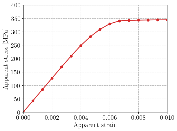
We plot the evolution of the apparent vertical stress as a function of the imposed apparent strain. We observe a progressive onset of plasticity after a first elastic phase. The apparent stress then saturates, reaching a perfectly plastic plateau associated with plastic collapse of the plate.
plt.plot(Eyy, Force / Lx, "-oC3")
plt.xlabel("Apparent strain")
plt.ylabel("Apparent stress [MPa]")
plt.ylim(0, 400)
plt.show()
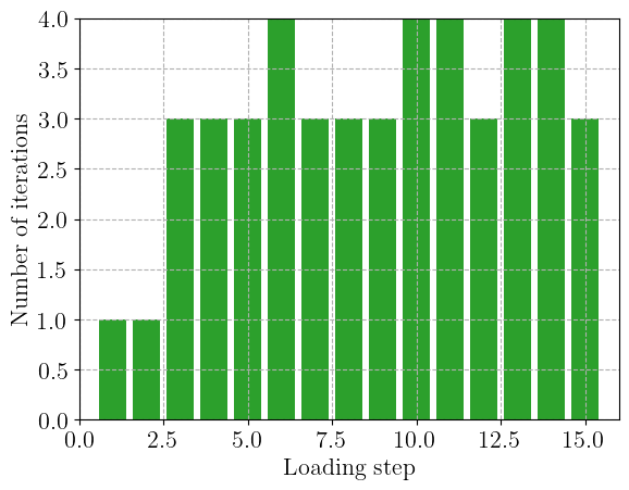
We report below the evolution of the number of Newton iterations for each load step. We can see that in the first iterations, convergence is reached in 1 iteration only, corresponding to the elastic stage. The number of iterations then increases during the plastic stage.
plt.bar(np.arange(N + 1), nit, color="C2")
plt.xlabel("Loading step")
plt.ylabel("Number of iterations")
plt.xlim(0, N + 1)
plt.show()
We measure below the time spent in the full SNES solve and the time spent only in the constitutive integration part. We can check that the latter represents only a small fraction of the total computing time which is mostly dominated by the cost of solving the global linear system at each global Newton iteration.
snes_solve = timing("SNES: solve")[1].total_seconds()
print(f"Total solving time {snes_solve:.2f}s")
constitutive_update_time = timing("SNES: constitutive update")[1].total_seconds()
print(f"Total time spent in constitutive update {constitutive_update_time:.2f}s")
Total solving time 20.81s
Total time spent in constitutive update 5.93s
We can list below the breakdown of the different timings.
list_timings(MPI.COMM_WORLD)
[MPI_MAX] Summary of timings (s)                                            |  reps       avg        tot
--------------------------------------------------------------------------------------------------------
Build dofmap data                                                           |    38  0.000547   0.020780
Compute connectivity 1-0                                                    |     1  0.000121   0.000121
Compute connectivity 2-0                                                    |     1  0.000009   0.000009
Compute dof reordering map                                                  |    38  0.000061   0.002309
Compute entities of dim = 1                                                 |     1  0.004229   0.004229
Compute local part of mesh dual graph (mixed)                               |     1  0.006600   0.006600
Compute local-to-local map                                                  |     1  0.000533   0.000533
Compute-local-to-global links for global/local adjacency list               |     1  0.000117   0.000117
Distribute row-wise data (scalable)                                         |     1  0.000124   0.000124
GPS: create_level_structure                                                 |     4  0.000264   0.001057
Gibbs-Poole-Stockmeyer ordering                                             |     1  0.002650   0.002650
Init dofmap from element dofmap                                             |    38  0.000348   0.013228
SNES: constitutive update                                                   |    61  0.097282   5.934185
SNES: solve                                                                 |    15  1.387307  20.809610
SparsityPattern::finalize                                                   |    31  0.000894   0.027722
Topology: create                                                            |     1  0.009592   0.009592
Topology: determine shared index ownership                                  |     1  0.000129   0.000129
Topology: determine vertex ownership groups (owned, undetermined, unowned)  |     1  0.000449   0.000449
dx_mat: External state variable update                                      |    62  0.000005   0.000284
dx_mat: Gradients evaluation                                                |    62  0.004550   0.282096
dx_mat: Material integration                                                |    62  0.153885   9.540887
dx_mat: Quadrature Expression evaluation                                    |    63  0.001970   0.124098
dx_mat: Update values and tangent operators                                 |    62  0.016279   1.009274
jaxmat: Constitutive update                                                 |    61  0.061609   3.758138
jaxmat: First pass (includes jit compilation)                               |     1  4.689493   4.689493
jaxmat: dolfinx to jaxmat conversion                                        |    62  0.008155   0.505586
jaxmat: jaxmat to dolfinx conversion                                        |    62  0.007902   0.489935