Linear elasticity#
Objectives
This demo shows how to define a linear problem, apply boundary conditions, solve for the solution and output to a results file. \(\newcommand{\bsig}{\boldsymbol{\sigma}} \newcommand{\beps}{\boldsymbol{\varepsilon}} \newcommand{\bu}{\boldsymbol{u}} \newcommand{\bv}{\boldsymbol{v}} \newcommand{\bT}{\boldsymbol{T}} \newcommand{\dOm}{\,\text{d}\Omega} \newcommand{\dS}{\,\text{d}S} \newcommand{\Neumann}{{\partial \Omega_\text{N}}} \newcommand{\Dirichlet}{{\partial \Omega_\text{D}}}\)
Download sources
Variational formulation#
Solving PDEs with FEniCSx requires to formulate the problem in weak or variational form. For a general introduction to variational formulations within the FEniCSx context, we refer the reader to https://jsdokken.com/dolfinx-tutorial/chapter1/fundamentals.html.
In the context of solid mechanics, the variational formulation within a small strain setting reads as:
Find \(\bu \in V\) such that:
\[\begin{equation*} \int_\Omega \bsig(\bu):\nabla^\text{s} \bv \dOm = \int_\Omega \boldsymbol{f}\cdot\bv \dOm + \int_\Neumann \bT\cdot\bv \dS \quad \forall \bv \in V_0 \end{equation*}\]
where \(\bu\) is the unknown displacement (the trial function) living in the space of admissible displacements \(V\) such that \(\bu=\bu_0\) on the Dirichlet boundary \(\Dirichlet\). \(\boldsymbol{f}\) and \(\bT\) are respectively body and surface traction forces. \(\sigma(\bu)\) is the Cauchy stress field which depends on the displacement \(\bu\). Finally, \(\bv\) denotes test functions living in the space of admissible perturbations \(V_0\) i.e. such that \(\bv=0\) on \(\Dirichlet\).
The above variational formulation represents the weak form of equilibrium and must be supplemented by a constitutive relation. In the linear elastic case, we have \(\bsig(\bu) = \mathbb{C}:\nabla^s \bu\) so that the above variational formulation reads:
Find \(\bu \in V\) such that:
\[\begin{equation*} \int_\Omega \nabla^\text{s}\bu:\mathbb{C}:\nabla^\text{s} \bv \dOm = \int_\Omega \boldsymbol{f}\cdot\bv \dOm + \int_\Neumann \bT\cdot\bv \dS \quad \forall \bv \in V_0 \end{equation*}\]
The left-hand side is a bilinear form of \(\bu\) and \(\bv\) whereas the right-hand side is a linear form. The above equality is generally written as \(a(\bu,\bv) = L(\bv)\quad \forall \bv \in V_0\).
The power of FEniCS is precisely to easily define such forms using symbolic expressions. After choosing a finite-element approximation for the test and trial function spaces, it will automatically generate code to compute the corresponding global stiffness matrix (for \(a\)) and vector of nodal forces (for \(L\)).
Implementation#
Relevant packages#
UFL: Symbolic expressions involved in the above expressions are handled by the
ufl(Unified Form Language] package which allows to combine abstract operators in a notation close to the mathematical one. UFL also provide theTestFunctionandTrialFunctionobjects appearing as arguments of linear or bilinear forms.DOLFINx: The
dolfinxpackage is the Python interface to the computational environment of FEniCSx. It provides all the necessary tools to load meshes, handle data structures and functions related to finite-elements (global FE function spaces and associated functions, assembling procedures, boundary conditions, solvers, etc.).other packages may include
mpi4pyfor MPI parallel communication,petsc4pyfor interaction with PETSc objects,ffcxfor Just-In-Time compilation of forms, etc.
Problem definition#
We will model a 2D rectangular beam of dimensions \(10\times 1\) which we will mesh with quadrangles. We first start by loading the relevant packages and functions. The dolfinx.mesh module provides a customary function for meshing a rectangular domain. For more complex cases, we can import meshes generated by external tools such as GMSH for instance.
import numpy as np
from ufl import sym, grad, Identity, tr, inner, Measure, TestFunction, TrialFunction

from mpi4py import MPI

from dolfinx import fem, io
import dolfinx.fem.petsc
from dolfinx.mesh import create_rectangle, CellType

length, height = 10, 1.0
Nx, Ny = 50, 5
domain = create_rectangle(
    MPI.COMM_WORLD,
    [np.array([0, 0]), np.array([length, height])],
    [Nx, Ny],
    cell_type=CellType.quadrilateral,
)

dim = domain.topology.dim
print(f"Mesh topology dimension d={dim}.")
Mesh topology dimension d=2.
Next, we define the finite-element FunctionSpace for our wanted solution u_sol. Here, we use a vector function space of type "P" (Polynomial), which implies standard Lagrange elements of degree deg=2 here.
Note
The keyword "Lagrange" also works instead of "P".
Deprecated since version 0.7: The definition of Function Spaces has slightly changed.
VectorFunctionSpaceandTensorFunctionSpaceare now deprecated and we must pass instead a shape argument when creating a standard function space.We should no longer use the class initializer
FunctionSpaceas this is meant for internal use only. We must now use the functionfunctionspaceinstead.You may also find in some older demos the keyword
"CG"(Continuous Galerkin) which is now deprecated.
degree = 2
shape = (dim,)  # this means we want a vector field of size `dim`
V = fem.functionspace(domain, ("P", degree, shape))

u_sol = fem.Function(V, name="Displacement")
INFO: Disabling color, you really want to install colorlog.
We now define the various UFL expressions which will enter our variational formulation. For this, we wrap material parameters as Constant.
E = fem.Constant(domain, 210e3)
nu = fem.Constant(domain, 0.3)

lmbda = E * nu / (1 + nu) / (1 - 2 * nu)
mu = E / 2 / (1 + nu)


def epsilon(v):
    return sym(grad(v))


def sigma(v):
    return lmbda * tr(epsilon(v)) * Identity(dim) + 2 * mu * epsilon(v)
We can check that such objects are indeed abstract UFL expressions (they are represented as graphs internally).
print("mu (UFL):\n", mu)
print("epsilon (UFL):\n", epsilon(u_sol))
print("sigma (UFL):\n", sigma(u_sol))
mu (UFL):
 c_0 / 2 / (1 + c_1)
epsilon (UFL):
 sym(grad(Displacement))
sigma (UFL):
 ({ A | A_{i_{10}, i_{11}} = (sym(grad(Displacement)))[i_{10}, i_{11}] * 2 * c_0 / 2 / (1 + c_1) }) + ({ A | A_{i_8, i_9} = I[i_8, i_9] * c_0 * c_1 / (1 + c_1) / (1 + -1 * 2 * c_1) * (tr(sym(grad(Displacement)))) })
We now define the corresponding linear and bilinear forms. Below, dx is the volume integration measure on the whole domain.
u = TrialFunction(V)
v = TestFunction(V)

rho = 2e-3
g = 9.81
f = fem.Constant(domain, np.array([0, -rho * g]))

dx = Measure("dx", domain=domain)
a = inner(sigma(u), epsilon(v)) * dx
L = inner(f, v) * dx
We now define boundary conditions. For simplicity, we first fix both the left and right boundaries. To do so, we must locate the corresponding degrees of freedom from a marker function thet returns True for points x on the boundary and False otherwise.
def left(x):
    return np.isclose(x[0], 0)


def right(x):
    return np.isclose(x[0], length)


left_dofs = fem.locate_dofs_geometrical(V, left)
right_dofs = fem.locate_dofs_geometrical(V, right)

bcs = [
    fem.dirichletbc(np.zeros((2,)), left_dofs, V),
    fem.dirichletbc(np.zeros((2,)), right_dofs, V),
]
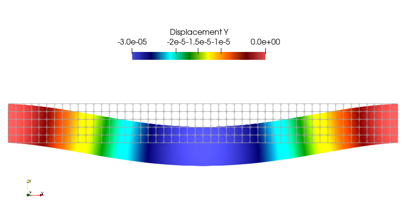
Finally, a LinearProblem object is created based on the variational problem, the boundary conditions and a Function u in which we want to store the solution. We can also pass parameters to setup the solver type (here we use a direct LU factorization).
Results are then stored in a “.pvd” format to be visualized using Paraview for instance.
problem = fem.petsc.LinearProblem(
    a, L, u=u_sol, bcs=bcs, petsc_options={"ksp_type": "preonly", "pc_type": "lu"}
)
problem.solve()


vtk = io.VTKFile(domain.comm, "linear_elasticity.pvd", "w")
vtk.write_function(u_sol)
vtk.close()
Changing boundary conditions#
If we want to constrain only the vertical component of the displacement field on some boundary, we need to work with the corresponding subspace of the original function space V.
V_uy, mapping = V.sub(1).collapse()
right_dofs_uy = fem.locate_dofs_geometrical((V.sub(1), V_uy), right)

uD_y = fem.Function(V_uy)
bcs2 = [
    fem.dirichletbc(np.zeros((2,)), left_dofs, V),
    fem.dirichletbc(uD_y, right_dofs_uy, V.sub(1)),
]

problem = fem.petsc.LinearProblem(
    a, L, u=u_sol, bcs=bcs2, petsc_options={"ksp_type": "preonly", "pc_type": "lu"}
)
problem.solve()


vtk = io.VTKFile(domain.comm, "linear_elasticity.pvd", "w")
vtk.write_function(u_sol)
vtk.close()
Exercise: thermal strains#
We consider the presence of thermal strains \(\beps^\text{th} = \alpha \Delta T(\boldsymbol{x}) \boldsymbol{I}\) where \(\Delta T(\boldsymbol{x})\) varies linearly from 0 to +20° between the bottom and top face of the beam. The stress-strain constitutive relation is now:
Implement a spatially dependent expression for \(\Delta T\) using
x = ufl.SpatialCoordinate(domain)for the position vectorx.Change the definition of the stress-strain relation and compute the corresponding linear and bilinear form.
Solve the problem with only the left boundary being fixed.
Hint
You can use the UFL functions ufl.lhs/ufl.rhs to extract the bilinear form (lhs), resp. the linear form (rhs), of a UFL expression containing both bilinear and linear forms.
from ufl import lhs, rhs, SpatialCoordinate

alp = fem.Constant(domain, 1e-5)
x = SpatialCoordinate(domain)