Generating a shell model with the Gmsh Python API #
Objectives
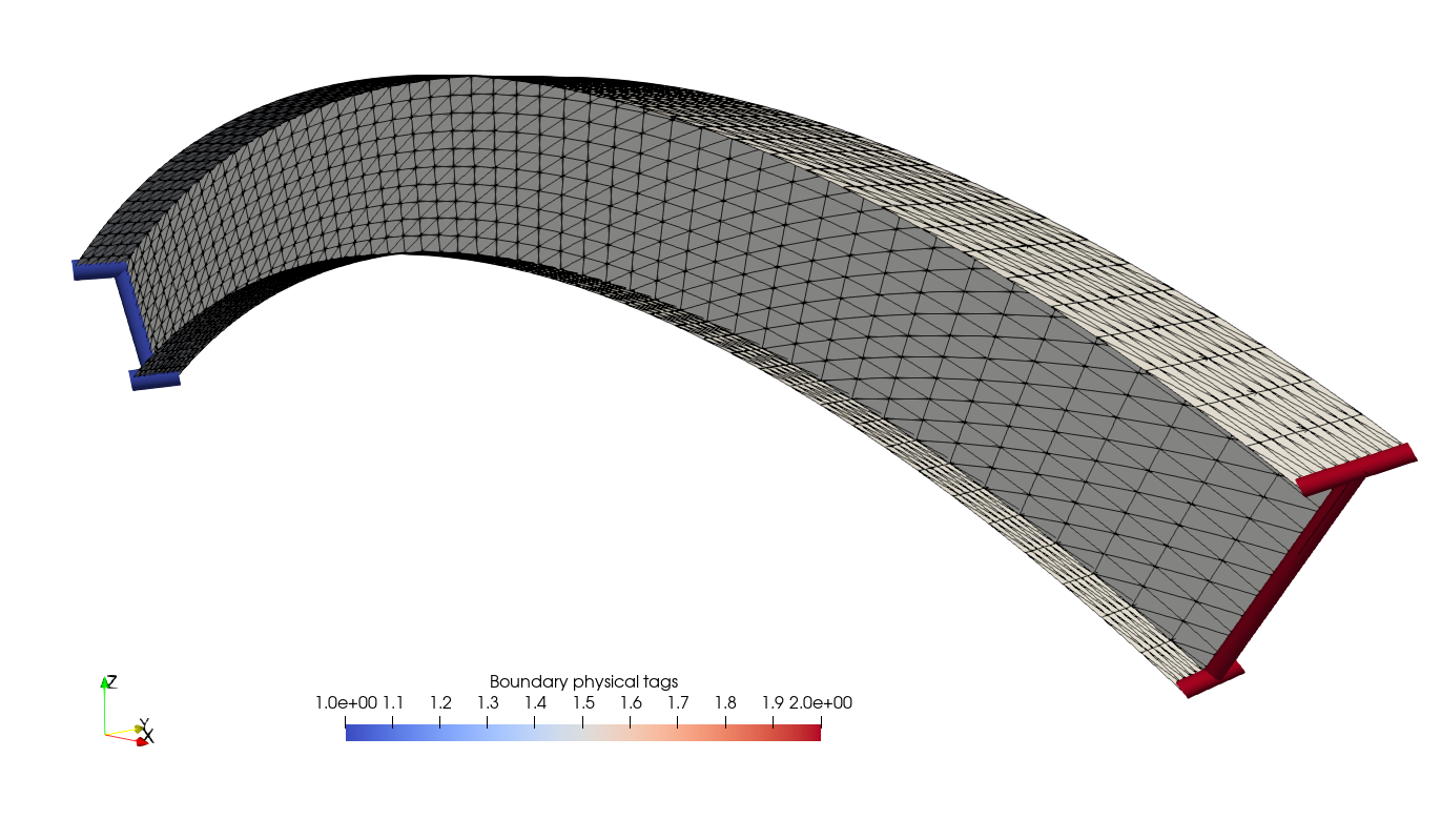
This notebook illustrates the use of the Gmsh Python API for generating a shell model of a curved I-beam model.
Download sources
Geometric parameters#
We consider a I-shaped constant cross-section for the beam with bottom and top flange widths wb and wt and of height h. The arch will be a portion of a circular arc of total angle opening \(2\theta\) and chord length \(L\). The circular arc radius is therefore given by \(R=\dfrac{L}{2\sin(\theta)}\) and the arch rise by \(f=R-\dfrac{L}{2\tan(\theta)}\).
import gmsh
import numpy as np

filename = "I_beam"
# I-beam profile
wb = 0.2  # bottom flange width
wt = 0.3  # top flange width
h = 0.5  # web height
# Arch geometry
theta = np.pi / 6  # arch opening half-angle
L = 10.0  # chord length
R = L / 2 / np.sin(theta)  # arch radius
f = R - L / 2 / np.tan(theta)  # arch rise
Defining points and lines for the left-hand side cross-section#
We first begin by initializing Gmsh ang use the built-in geo CAD kernel since we won’t require any boolean operation which require the use of the Open Cascade kernel.
gmsh.initialize()
geom = gmsh.model.geo
Next, we define the points and lines of the left-hand side cross-section. To facilitate their definition, these objects are first defined for a vertical cross-section located in the \(X=0\) plane and centered on the origin \((0,0,0)\). We split them into a group of bottom_points for the bottom_flange and a group of top_points for the top_flange. The web then connects the middle points of each group. The start_section contains the web, bottom and top flange lines.
Note
Note that Gmsh requires passing a mesh density for each point definition. However, this lcar value will not be used in the end since we will later define the number of points on each line using the TransfiniteCurve command.
lcar = 0.1  # characteristic mesh size density (will not be used)
bottom_points = [
    geom.addPoint(0, -wb / 2, -h / 2, lcar),
    geom.addPoint(0, 0, -h / 2, lcar),
    geom.addPoint(0, wb / 2, -h / 2, lcar),
]
top_points = [
    geom.addPoint(0, -wt / 2, h / 2, lcar),
    geom.addPoint(0, 0, h / 2, lcar),
    geom.addPoint(0, wt / 2, h / 2, lcar),
]
bottom_flange = [
    geom.addLine(bottom_points[0], bottom_points[1]),
    geom.addLine(bottom_points[1], bottom_points[2]),
]
web = [geom.addLine(bottom_points[1], top_points[1])]
top_flange = [
    geom.addLine(top_points[0], top_points[1]),
    geom.addLine(top_points[1], top_points[2]),
]
start_section = bottom_flange + web + top_flange
Cross-section rotation and extrusion#
Now, we rotate this section by an angle equal to \(-\theta\) around the \(Y\) axis to obtain our initial starting section for the arch. The rotate command requires a dimTags first argument i.e. a list of tuple of the form (dim, label) where dim is the entity dimension (dim=1 here for lines) and label is the label entity. The following arguments are then x, y, z, ax, ay, az, angle defining a rotation of angle angle around an axis of revolution passing through a point (x, y, z) along a direction (ax, ay, az).
dimTags = [(1, l) for l in start_section]
geom.rotate(dimTags, 0, 0, 0, 0, 1, 0, -theta)
We will now extrude the previously defined cross-section along a circular arc. The extrude command is used for extruding along a line, here we will need the ̀revolve command to extrude the cross-section by following a rotation of angle \(2\theta\) which is defined similarly to the rotate command. Here, the axis follows the direction \((0, 1, 0)\) and passes through the point \((L/2, 0, -(R-f))\). We also pass a list of layers and corresponding numbers of elements generated during extrusion. Here, we have only one layer (normalized height = 1.0) of 50 elements.
The revolve command returns a list of dimTags corresponding to the newly created entities. For instance, when extruding a line, this will create a surface and three new lines. The output stores these entities as follows:
\([\text{end line}, \text{ surface}, \text{ lateral line }1,\text{ lateral line }2]\). We loop on the various entities composing the starting cross-section and append the newly created end-lines and surfaces in corresponding lists. Note that we need to call synchronize to update the corresponding Gmsh model with the newly created entities.
end_bottom_flange = []
end_top_flange = []
end_web = []
surfaces = []
for ini, end in zip(
    [bottom_flange, web, top_flange], [end_bottom_flange, end_web, end_top_flange]
):
    for l in ini:
        outDimTags = geom.revolve(
            [(1, l)],
            L / 2,
            0,
            -(R - f),
            0,
            1,
            0,
            2 * theta,
            numElements=[50],
            heights=[1.0],
        )
        end.append(outDimTags[0][1])
        surfaces.append(outDimTags[1][1])
        geom.synchronize()
end_section = end_bottom_flange + end_web + end_top_flange
Tagging and mesh generation#
We finish by specifying the number of elements for the flange and web discretization using the setTransfiniteCurve command. We also affect the physical tag 1 for the left-hand side cross-section and 2 for the right-hand side cross section. We do not forget to also add physical tags to the surfaces otherwise they well later be ignored when generating the mesh.
for f in bottom_flange + top_flange + end_bottom_flange + end_top_flange:
    geom.mesh.setTransfiniteCurve(f, 6)
for w in web + end_web:
    geom.mesh.setTransfiniteCurve(w, 11)

gmsh.model.addPhysicalGroup(2, surfaces, 1)
gmsh.model.addPhysicalGroup(1, start_section, 1)
gmsh.model.addPhysicalGroup(1, end_section, 2)
2
We can now call the mesh generate function (up to dimension dim=2 since we don’t have any 3D solid element here). The generated mesh is then exported to a .msh. We finish by the finalize command since we are finished with the Gmsh API.
Tip
You can export the corresponding geo file by writing to a file with a .geo_unrolled extension.
gmsh.model.mesh.generate(dim=2)
gmsh.write(filename + ".msh")

gmsh.finalize()
Info    : Meshing 1D...
Info    : [  0%] Meshing curve 1 (Line)
Info    : [ 10%] Meshing curve 2 (Line)
Info    : [ 20%] Meshing curve 3 (Line)
Info    : [ 20%] Meshing curve 4 (Line)
Info    : [ 30%] Meshing curve 5 (Line)
Info    : [ 40%] Meshing curve 6 (Extruded)
Info    : [ 40%] Meshing curve 7 (Extruded)
Info    : [ 50%] Meshing curve 8 (Extruded)
Info    : [ 50%] Meshing curve 10 (Extruded)
Info    : [ 60%] Meshing curve 12 (Extruded)
Info    : [ 70%] Meshing curve 14 (Extruded)
Info    : [ 70%] Meshing curve 16 (Extruded)
Info    : [ 80%] Meshing curve 18 (Extruded)
Info    : [ 90%] Meshing curve 19 (Extruded)
Info    : [ 90%] Meshing curve 22 (Extruded)
Info    : [100%] Meshing curve 24 (Extruded)
Info    : Done meshing 1D (Wall 0.000240038s, CPU 0.000352s)
Info    : Meshing 2D...
Info    : [  0%] Meshing surface 9 (Extruded)
Info    : [ 20%] Meshing surface 13 (Extruded)
Info    : [ 40%] Meshing surface 17 (Extruded)
Info    : [ 60%] Meshing surface 21 (Extruded)
Info    : [ 80%] Meshing surface 25 (Extruded)
Info    : Done meshing 2D (Wall 0.00232941s, CPU 0.001437s)
Info    : 617 nodes 1439 elements
Info    : Writing 'I_beam.msh'...
Info    : Done writing 'I_beam.msh'