Shear-locking in thick plate models with quadrilateral elements #
Objectives
This tour implements a thick plate Reissner-Mindlin model and discusses the issue of shear-locking in the thin plate limit. We show how to use selective reduced integration to alleviate this issue.
Download sources
See also
For more details on the Reissner-Mindlin plate model and its implementation, we refer to the Reissner-Mindlin plates introductory tour.
See also
For more advanced Reissner-Mindlin plate elements, we refer to FEniCSx-Shells.
Introduction#
This program solves the Reissner-Mindlin plate equations on the unit square with uniform transverse loading and fully clamped boundary conditions. We will test the use of quadrilateral cells and selective reduced integration (SRI) to remove shear-locking issues in the thin plate limit. Both linear and quadratic interpolation are considered for the transverse deflection \(w\) and rotation \(\boldsymbol{\theta}\).
Implementation#
We first create a unit square mesh divided in \(N\times N\) quadrilaterals:
import numpy as np
from mpi4py import MPI
import ufl
import basix
from dolfinx import fem, mesh
import dolfinx.fem.petsc

N = 50
domain = mesh.create_unit_square(MPI.COMM_WORLD, N, N, mesh.CellType.quadrilateral)
Material parameters for isotropic linear elastic behavior are first defined:
E = fem.Constant(domain, 210e3)
nu = fem.Constant(domain, 0.3)
Plate bending stiffness \(\textsf{D}=\dfrac{Eh^3}{12(1-\nu^2)}\) and shear stiffness \(\textsf{F} = \kappa G h\) with a shear correction factor \(\kappa = 5/6\) for a homogeneous plate of thickness \(h\):
thick = fem.Constant(domain, 1e-3)
D = E * thick**3 / (1 - nu**2) / 12.0
F = E / 2 / (1 + nu) * thick * 5.0 / 6.0
The uniform loading \(f\) is scaled by the Love-Kirchhoff solution so that the deflection converges to a constant value of 1 in the thin plate. This thin plate limit will be used to check the sensitivity of the element to shear locking. Formulations which exhibit shear locking are expected to provide overly stiff results (low values of the deflection) for a given mesh in the limit of small thickness \(h \to 0\).
f = -D / 1.265319087e-3 # with this we have w_Love-Kirchhoff = 1.0
Continuous interpolation using degree \(d=\texttt{deg}\) is chosen for both deflection and rotation. Note that when using quadrilaterals, we have different choices of interpolation over the cell. We will not discuss here variants such as equispaced or GLL variants which mostly differ in the dof location up to \(d=3\), see here for more details. However, already for \(d=2\), we may have the choice of using an 8 or a 9-dof quadrilateral.
name="S", it has 8 dofs, spanning polynomials up to order 2, except for \(x^2y^2\)
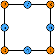
see details here
name="Q", it has 9 dofs, spanning polynomials up to order 2, including \(x^2y^2\)
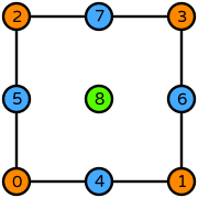
see details here
deg = 2
el_type = "S"  # or "Q"
We = basix.ufl.element(el_type, domain.basix_cell(), deg)
Te = basix.ufl.element(el_type, domain.basix_cell(), deg, shape=(2,))
V = fem.functionspace(domain, basix.ufl.mixed_element([We, Te]))
Clamped boundary conditions on the lateral boundary are defined as:
# Boundary of the plate
def border(x):
    return np.logical_or(
        np.logical_or(np.isclose(x[0], 0), np.isclose(x[0], 1)),
        np.logical_or(np.isclose(x[1], 0), np.isclose(x[1], 1)),
    )


facet_dim = 1
clamped_facets = mesh.locate_entities_boundary(domain, facet_dim, border)
clamped_dofs = fem.locate_dofs_topological(V, facet_dim, clamped_facets)

u0 = fem.Function(V)
bcs = [fem.dirichletbc(u0, clamped_dofs)]
Some useful functions for implementing generalized constitutive relations are now defined:
def strain2voigt(eps):
    return ufl.as_vector([eps[0, 0], eps[1, 1], 2 * eps[0, 1]])


def voigt2stress(S):
    return ufl.as_tensor([[S[0], S[2]], [S[2], S[1]]])


def curv(u):
    (w, theta) = ufl.split(u)
    return ufl.sym(ufl.grad(theta))


def shear_strain(u):
    (w, theta) = ufl.split(u)
    return ufl.grad(w) - theta


def bending_moment(u):
    DD = ufl.as_tensor([[D, nu * D, 0], [nu * D, D, 0], [0, 0, D * (1 - nu) / 2.0]])
    return voigt2stress(ufl.dot(DD, strain2voigt(curv(u))))


def shear_force(u):
    return F * shear_strain(u)
The contribution of shear forces to the total energy is under-integrated using a custom quadrature rule of degree \(2d-2\) i.e. for linear (\(d=1\)) quadrilaterals, the shear energy is integrated as if it were constant (1 Gauss point instead of 2x2) and for quadratic (\(d=2\)) quadrilaterals, as if it were quadratic (2x2 Gauss points instead of 3x3).
See also
See the Quadrature schemes tour for more details on the choice of quadrature points.
u = fem.Function(V)
u_ = ufl.TestFunction(V)
du = ufl.TrialFunction(V)

dx = ufl.Measure("dx")
dx_shear = ufl.Measure("dx", metadata={"quadrature_degree": 2 * deg - 2})

L = f * u_[0] * dx
a = (
    ufl.inner(bending_moment(u_), curv(du)) * dx
    + ufl.dot(shear_force(u_), shear_strain(du)) * dx_shear
)
We then solve for the solution and print the deflection normalized with respect to the Love-Kirchhoff thin plate analytical solution:
problem = fem.petsc.LinearProblem(
    a, L, u=u, bcs=bcs, petsc_options={"ksp_type": "preonly", "pc_type": "lu"}
)
problem.solve()

w = u.sub(0).collapse()
w.name = "Deflection"

print(f"Reissner-Mindlin FE deflection: {max(abs(w.vector.array)):.5f}")
Reissner-Mindlin FE deflection: 1.00002
Results#
We provide here some results for \(h=0.001\) using either \(N=10\) or \(N=50\) quads per side and for different types of interpolation and integration.
Type |
\(N=10\) |
\(N=50\) |
|---|---|---|
|
0.00046 |
0.01116 |
|
0.99261 |
0.99972 |
|
0.72711 |
0.99864 |
|
0.87658 |
1.00002 |
|
0.96450 |
0.99865 |
|
1.00021 |
1.00002 |
The results show that the low-order elements \(d=1\) always lock very strongly but accurate estimates are obtained using selective reduced integration (SRI). The Serendipity element S exhibits a notable locking behavior which is not necessarily fixed using SRI. On the contrary, for Q elements, locking is less pronounced and the behavior of the element is improved when using SRI.