Reissner-Mindlin plates#
Objectives
This demo illustrates how to implement a Reissner-Mindlin thick plate model. The main specificity of such models is that one needs to solve for two different fields: a vertical deflection field \(w\) and a rotation vector field \(\boldsymbol{\theta}\). \(\newcommand{\bM}{\boldsymbol{M}} \newcommand{\bQ}{\boldsymbol{Q}} \newcommand{\bgamma}{\boldsymbol{\gamma}} \newcommand{\btheta}{\boldsymbol{\theta}} \newcommand{\bchi}{\boldsymbol{\chi}} \renewcommand{\div}{\operatorname{div}}\)

Download sources
Governing equations#
We recall below the main relations defining this model in the linear elastic case.
Generalized strains#
Bending curvature strain \(\bchi = \dfrac{1}{2}(\nabla \btheta + \nabla^\text{T} \btheta) = \nabla^\text{s}\btheta\)
Shear strain \(\bgamma = \nabla w - \btheta\)
Generalized stresses#
Bending moment \(\bM\)
Shear force \(\bQ\)
Equilibrium conditions#
For a distributed transverse surface loading \(f\),
Vertical equilibrium: \(\div \bQ + f = 0\)
Moment equilibrium: \(\div \bM + \bQ = 0\)
In weak form:
Isotropic linear elastic constitutive relation#
Bending/curvature relation: \begin{align*} \begin{Bmatrix}M_{xx}\ M_{yy} \M_{xy} \end{Bmatrix} &= \textsf{D} \begin{bmatrix}1 & \nu & 0 \ \nu & 1 & 0 \ 0 & 0 & (1-\nu)/2 \end{bmatrix}\begin{Bmatrix}\chi_{xx} \ \chi_{yy} \ 2\chi_{xy} \end{Bmatrix}\ \text{ where}\quad \textsf{D} &= \dfrac{E h^3}{12(1-\nu^2)} \end{align*}
Shear strain/stress relation: \begin{align*} \bQ &= \textsf{F}\bgamma\ \text{ where}\quad \textsf{F} &= \dfrac{5}{6}\dfrac{E h}{2(1+\nu)} \end{align*}
Implementation#
We first load relevant modules and functions and generate a unit square mesh of triangles.
import numpy as np
import ufl
import basix

from mpi4py import MPI
from dolfinx import fem, io
import dolfinx.fem.petsc
from dolfinx.mesh import (
    create_unit_square,
    CellType,
    DiagonalType,
    locate_entities_boundary,
)


N = 10
domain = create_unit_square(
    MPI.COMM_WORLD, N, N, cell_type=CellType.triangle, diagonal=DiagonalType.crossed
)
Next we define material properties and functions which will be used for defining the variational formulation.
# material parameters
thick = 0.05
E = 210.0e3
nu = 0.3

# bending stiffness
D = fem.Constant(domain, E * thick**3 / (1 - nu**2) / 12.0)
# shear stiffness
F = fem.Constant(domain, E / 2 / (1 + nu) * thick * 5.0 / 6.0)

# uniform transversal load
f = fem.Constant(domain, -100.0)


# Useful function for defining strains and stresses
def curvature(u):
    (w, theta) = ufl.split(u)
    return ufl.as_vector(
        [theta[0].dx(0), theta[1].dx(1), theta[0].dx(1) + theta[1].dx(0)]
    )


def shear_strain(u):
    (w, theta) = ufl.split(u)
    return ufl.grad(w) - theta


def bending_moment(u):
    DD = ufl.as_matrix([[D, nu * D, 0], [nu * D, D, 0], [0, 0, D * (1 - nu) / 2.0]])
    return ufl.dot(DD, curvature(u))


def shear_force(u):
    return F * shear_strain(u)
Now we define the corresponding function space. Our dofs are \(w\) and \(\btheta\), so the full function space \(V\) will be a mixed function space consisting of a scalar subspace related to \(w\) and a vectorial subspace related to \(\btheta\). We first use a continuous \(P^2\) interpolation for \(w\) and a continuous \(P^1\) interpolation for \(\btheta\). We then define the corresponding linear and bilinear forms.
# Definition of function space for U:displacement, T:rotation
Ue = basix.ufl.element("P", domain.basix_cell(), 2)
Te = basix.ufl.element("P", domain.basix_cell(), 1, shape=(2,))
V = fem.functionspace(domain, basix.ufl.mixed_element([Ue, Te]))

# Functions
u = fem.Function(V, name="Unknown")
u_ = ufl.TestFunction(V)
(w_, theta_) = ufl.split(u_)
du = ufl.TrialFunction(V)

# Linear and bilinear forms
dx = ufl.Measure("dx", domain=domain)
L = f * w_ * dx
a = (
    ufl.dot(bending_moment(u_), curvature(du))
    + ufl.dot(shear_force(u_), shear_strain(du))
) * dx
Boundary conditions are now defined. We consider a fully clamped boundary. Note that since we are using a mixed function space, we cannnot use the locate_dofs_geometrical function. Instead, we locate the facets on the boundary using dolfinx.mesh.locate_entities_boundary. Then we locate the dofs on such facets using locate_dofs_topological.
# Boundary of the plate
def border(x):
    return np.logical_or(
        np.logical_or(np.isclose(x[0], 0), np.isclose(x[0], 1)),
        np.logical_or(np.isclose(x[1], 0), np.isclose(x[1], 1)),
    )


facet_dim = 1
clamped_facets = locate_entities_boundary(domain, facet_dim, border)
clamped_dofs = fem.locate_dofs_topological(V, facet_dim, clamped_facets)

u0 = fem.Function(V)
bcs = [fem.dirichletbc(u0, clamped_dofs)]
We now solve the problem and output the result. To get the deflection \(w\), we use u.sub(0).collapse() to extract a new function living in the corresponding subspace. Note that u.sub(0) provides only an indexed view of the \(w\) component of u. The computed results is compared with the analytical maximum deflection of a clamped Love-Kirchhoff plate:
problem = fem.petsc.LinearProblem(
    a, L, u=u, bcs=bcs, petsc_options={"ksp_type": "preonly", "pc_type": "lu"}
)
problem.solve()

with io.VTKFile(domain.comm, "plates.xdmf", "w") as vtk:
    w = u.sub(0).collapse()
    w.name = "Deflection"
    vtk.write_function(w)

w_LK = 1.265319087e-3 * -f.value / D.value
print(f"Reissner-Mindlin deflection: {max(abs(w.vector.array)):.5f}")
print(f"Love-Kirchhoff deflection: {w_LK:.5f}")
Reissner-Mindlin deflection: 0.05380
Love-Kirchhoff deflection: 0.05264
Warning
This simple formulation may suffer from shear locking issues in the thin plate limit. We refer to the various plate tours dedicated to this specific issue for more accurate treatment of plate shear locking.
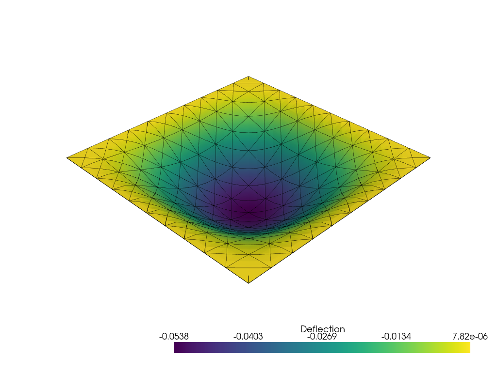
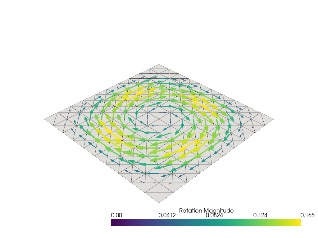
We can plot the plate deflection \(w\) and the rotation vector \(\boldsymbol{\beta} = \boldsymbol{e}_z\times \btheta\) using pyvista. \(\boldsymbol{\beta}\) represents the axis vector around which the plate is rotating.
Show code cell source
import pyvista
from dolfinx import plot

pyvista.set_jupyter_backend("static")

Vw = w.function_space
w_topology, w_cell_types, w_geometry = plot.vtk_mesh(Vw)
w_grid = pyvista.UnstructuredGrid(w_topology, w_cell_types, w_geometry)
w_grid.point_data["Deflection"] = w.x.array
w_grid.set_active_scalars("Deflection")
warped = w_grid.warp_by_scalar("Deflection", factor=5)

plotter = pyvista.Plotter()
plotter.add_mesh(
    warped,
    show_scalar_bar=True,
    scalars="Deflection",
)
edges = warped.extract_all_edges()
plotter.add_mesh(edges, color="k", line_width=1)
plotter.show()

theta = u.sub(1).collapse()
Vt = theta.function_space
theta_topology, theta_cell_types, theta_geometry = plot.vtk_mesh(Vt)
theta_grid = pyvista.UnstructuredGrid(theta_topology, theta_cell_types, theta_geometry)
beta_3D = np.zeros((theta_geometry.shape[0], 3))
beta_3D[:, :2] = theta.x.array.reshape(-1, 2) @ np.array([[0, -1], [1, 0]])
theta_grid["beta"] = beta_3D
theta_grid.set_active_vectors("beta")

plotter = pyvista.Plotter()
plotter.add_mesh(
    theta_grid.arrows, lighting=False, scalar_bar_args={"title": "Rotation Magnitude"}
)
plotter.add_mesh(theta_grid, color="grey", ambient=0.6, opacity=0.5, show_edges=True)
plotter.show()
Modal analysis#
Now we define the form corresponding to the definition of the mass matrix and we assemble the stiffness and mass forms into corresponding PETSc matrix objects. We use a value of 1 on the diagonal for K and 0 for M for the rows corresponding to the boundary conditions. Doing so, eigenvalues associated to boundary conditions are equal to infinity and will not pollute the low-frequency spectrum.
rho = fem.Constant(domain, 2700.0)
m_form = rho * thick * ufl.dot(du, u_) * dx

K = fem.petsc.assemble_matrix(fem.form(a), bcs, diagonal=1)
K.assemble()
M = fem.petsc.assemble_matrix(fem.form(m_form), bcs, diagonal=0)
M.assemble()
We now use slepc4py to define a eigenvalue solver (EPS – Eigenvalue Problem Solver – in SLEPc vocable) and solve the corresponding generalized eigenvalue problem. Functions defined in eigenvalue_solver.py
enable to define the corresponding objects, set up the parameters, monitor the resolution and extract the corresponding eigenpairs. Here the problem is of type GHEP (Generalized Hermitian eigenproblem) and we use a shift-invert transform to compute the smallest eigenvalues.
from slepc4py import SLEPc
from eigenvalue_solver import solve_GEP_shiftinvert, EPS_get_spectrum

N_eig = 6  # number of requested eigenvalues
eigensolver = solve_GEP_shiftinvert(
    K,
    M,
    problem_type=SLEPc.EPS.ProblemType.GHEP,
    solver=SLEPc.EPS.Type.KRYLOVSCHUR,
    nev=N_eig,
)
# Extract results
(eigval, eigvec_r, eigvec_i) = EPS_get_spectrum(eigensolver, V)
# Output eigenmodes
with io.VTKFile(domain.comm, "plates_eigenvalues.xdmf", "w") as vtk:
    for i in range(N_eig):
        w = eigvec_r[i].sub(0).collapse()
        w.name = "Deflection"
        vtk.write_function(w, i)
******************************
***  SLEPc Iterations...   ***
******************************
Iter. | Conv. | Max. error
    1 |     3 | 5.6e-06
    2 |     7 | 3.0e-07

******************************
*** SLEPc Solution Results ***
******************************
Iteration number: 2
Converged eigenpairs: 7

Converged eigval.  Error
----------------- -------
 9.12e-01             2.1e-12
 1.67e+00             7.1e-10
 1.67e+00             6.7e-13
 2.34e+00             1.2e-09
 2.89e+00             2.8e-13
 3.15e+00             3.4e-13
 3.56e+00             4.7e-12
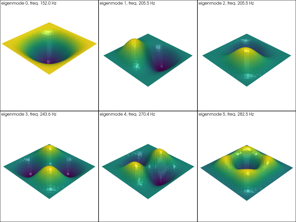
The eigenmodes look as follows using pyvista:
Show code cell source
w_grid = pyvista.UnstructuredGrid(w_topology, w_cell_types, w_geometry)

pl = pyvista.Plotter(shape=(2, 3))
for i in range(2):
    for j in range(3):
        pl.subplot(i, j)
        current_index = 3 * i + j
        eigenmode = f"eigenmode_{current_index:02}"
        pl.add_text(
            f"eigenmode {current_index}, freq. {np.real(np.sqrt(eigval[current_index]))/2/np.pi*1e3:.1f} Hz",
            font_size=10,
        )
        wi = eigvec_r[current_index].sub(0).collapse()
        w_grid[eigenmode] = wi.x.array
        pl.add_mesh(
            w_grid.warp_by_scalar(eigenmode, factor=10.0),
            scalars=eigenmode,
            show_scalar_bar=False,
            specular=0.5,
            specular_power=30,
        )
pl.show()