Localized 1D solutions in phase-field approach to brittle fracture

Objectives

This demo demonstrates how to solve a bound-constrained PDE optimization problem using PETSc TAO solver. The application examples involves the computation of localized solutions in the phase-field/damage gradient approach to brittle fracture. \(\newcommand{\dOm}{\,\text{d}\Omega}\)

Download sources

• Python script

• Jupyter notebook

• Complete sources files

Introduction

Bound-constrained problems involve finding the optimal solution of optimization problems of the form:

\[\begin{split}\begin{array}{rl} \displaystyle{\min_{x\in\mathbb{R}^n}} & f(x)\\ \text{s.t.} & x_l \leq x \leq x_u \end{array}\end{split}\]

where \(f(x)\) is the objective function to minimize and \(x_l, x_u\) are known lower and upper bounds set on the optimization vector \(x\).

There exist many methods to solve such a constrained optimization problem. It is important to note that constraints are here very simple as they bound only the minimum and maximum values of the optimization variable \(x\). In particular, this setting does not allow for more general linear or non-linear equality or inequality constraints.

PETSc’s Toolkit for Advanced Optimization (TAO) offers a wide range of algorithms to solve various constrained or unconstrained optimization problems, including bound-constrained problems. To interact with such a solver, the user is required to provide the objective function and the bounds. Depending on the chosen algorithm, the user should also provide:

• the objective gradient \(\nabla f(x)\);

• the Hessian operator \(\nabla^2 f(x)\).

In the following demo, we will use

Problem position

We consider a simple 1D bound constrained problem which arise from the use of phase-field or damage gradient models of brittle fracture [Bourdin et al., 2000, Pham et al., 2011]. In such methods, we simulate the propagation of cracks by minimizing a total energy consisting of an elastic and a fracture energy. When using one of the classical models of the phase-field approach, namely the \(\text{AT1}\) model, the fracture energy is written as:

(25)\[\mathcal{E}_\text{f}(d) = \dfrac{3G_\text{c}}{8\ell_0}\int_{\Omega}\left(d + \ell_0^2\nabla d \cdot\nabla d\right)\dOm\]

where \(d\) is a damage-like variable (with values in \([0;1]\)) which smears the discrete crack representation (corresponding to \(d=1\)) over a regularization length \(\ell_0\). \(G_\text{c}\) represents the material fracture energy.

During the solution process, the damage field is found by minimizing the total energy for a fixed displacement field and subject to bound constraints \(d_n \leq d \leq 1\) where \(d_n\) denotes the damage field at the previous time step which is used to enforce the irreversible evolution of damage.

When subject to a given mechanical loading, damage field will tend to localize spatially, corresponding to a smeared crack representation. In the 1D setting, it is possible to characterize the shape of the localized solution by finding damage fields which minimize the fracture energy (25).

Localized 1D solutions

More precisely, we consider a 1D domain \(\Omega=[-L;L]\) of length \(2L\) and we look for a minimizer \(d(x)\) of:

(26)\[\begin{split}\begin{array}{rl} \displaystyle\min_{d(x)} & \displaystyle\int_{\Omega}\left(d + \ell_0^2\left(\dfrac{\partial d}{\partial x}\right)^2\right)\dOm \\ \text{s.t.} & 0 \leq d(x) \leq 1 \quad \forall x \in \Omega \end{array}\end{split}\]

where we ignored the factor \(3G_\text{c}/(8\ell_0)\) of the fracture energy. In the following, we note \(j(d)\) the objective function of (26).

In addition, in order to force localization around a given point, we will impose here the boundary condition \(d(x)=d_0\) at \(x=0\) where \(d_0\in [0;1]\) is given. In this case, we can show that there exists a region \(]-D;D[\) where \(0 < d(x) < 1\) and with \(d(x)=0\) outside. We can show in particular that we must have \(d(\pm D) = \dfrac{\partial d}{\partial x}(\pm D) = 0\) at the transition points [Pham et al., 2011, Pham and Marigo, 2013].

In the inner region, since the bounds are not attained, the optimal solution is characterized by the fact that the first variation of the objective is null, that is:

\[\begin{align*} D_d j(d;\widehat{d}) = 0 \quad \forall \widehat{d}\\ \int_{\Omega} \left(\widehat{d} + \ell_0^2 \dfrac{\partial d}{\partial x}\dfrac{\partial \widehat{d}}{\partial x}\right)\dOm = 0 \quad \forall \widehat{d}\\ \end{align*}\]

The corresponding linear variational problem results in the following strong form differential equation:

\[ \dfrac{\partial^2 d}{\partial x^2} = \dfrac{1}{2\ell_0^2} \]

Accounting for the following boundary conditions:

\[ d(0)=d_0 \quad ; \quad d(\pm D) = 0 \quad ;\quad \dfrac{\partial d}{\partial x}(\pm D) = 0 \]

we easily show that the localization region size is \(D=2\ell_0\sqrt{d_0}\) and that the solution is given by:

(27)\[\begin{split}d(x) = \begin{cases} \left(\sqrt{d_0} - \dfrac{|x|}{2\ell_0}\right)^2 & \text{if } |x| \leq D \\ 0 & \text{otherwise} \end{cases}\end{split}\]

Implementation

For the implementation, we first provide a utility class TAOProblem in the tao_problem.py module. This class enables to interact with PETSc TAO solver objects by providing methods for computing the objective function, the gradient and the Hessian/Jacobian of the objective.

We now import the relevant modules and define the 1D domain \(\Omega=[-L;L]\)

import numpy as np
import matplotlib.pyplot as plt
from petsc4py import PETSc
from mpi4py import MPI
import ufl
from dolfinx import fem, mesh
import dolfinx.fem.petsc
from tao_problem import TAOProblem

N = 40
L = 5.0
domain = mesh.create_interval(MPI.COMM_WORLD, 2 * N, [-L, L])

We now create a scalar \(\mathbb{P}_1\) Lagrange function space and defines functions to store the lower and upper bound values.

V = fem.functionspace(domain, ("P", 1))
d = fem.Function(V)
d_ = ufl.TestFunction(V)
dd = ufl.TrialFunction(V)
dlb = fem.Function(V, name="Lower_bound")
dlb.vector.set(0.0)
dub = fem.Function(V, name="Upper_bound")
dub.vector.set(1.0)

We define the boundary condition at \(x=0\).

def middle_node(x):
    return np.isclose(x[0], 0)


middle_dof = fem.locate_dofs_geometrical(V, middle_node)

d_imp = fem.Constant(domain, 0.0)
bcs = [fem.dirichletbc(d_imp, middle_dof, V)]

We now define the objective function to minimize, corresponding to the fracture energy up to a scaling factor. We also use ufl.derivative to compute automatically the first and second variations which will be used for setting the gradient and Hessian.

ell0 = fem.Constant(domain, 1.0)
energy = (d + ell0**2 * ufl.dot(ufl.grad(d), ufl.grad(d))) * ufl.dx
D_energy = ufl.derivative(energy, d, d_)
D2_energy = ufl.derivative(D_energy, d, dd)

Now, we instantiate the TAOProblem object by providing the objective function form and its first and second variations, the function d corresponding to the optimization variable and the associated boundary condition list.

problem = TAOProblem(energy, D_energy, D2_energy, d, bcs)

We now setup the TAO solver object using petsc4py. We use a Bounded Newton Line Search bnls method and use a direct LU solver for the resolution of linear systems arising in the underlying Newton method.

See also

For more details on the algorithm and other available solvers, see the bound-constrained solvers documentation.

tao = PETSc.TAO().create(PETSc.COMM_SELF)
tao.setType("bnls")
tao.getKSP().setType("preonly")
tao.getKSP().getPC().setType("lu")

We use the utility functions provided by the TAOProblem class to set the objective, the gradient and the Hessian.

tao.setObjective(problem.f)
tao.setGradient(problem.F, problem.b)
tao.setHessian(problem.J, problem.A)

Finally, we set the corresponding variable bounds and we also prescribe some stopping tolerances where:

\[\begin{align*} \texttt{gatol} &= \|\nabla f(X)\|\\ \texttt{grtol} &= \|\nabla f(X)\|/|f(X)|\\ \texttt{gttol} &= \|\nabla f(X)\|/ \|\nabla f(X_0)\| \end{align*}\]

with \(X_0\) being the initial value.

tao.setVariableBounds(dlb.vector, dub.vector)
tao.setTolerances(gatol=1e-6, grtol=1e-6, gttol=1e-6)

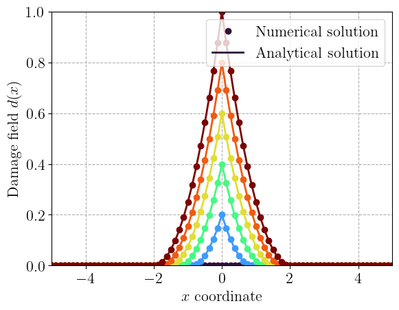
We now set different values of \(d_0 \in [0;1]\) and solve the corresponding problem.

values = np.linspace(0, 1.0, 6)
x = V.tabulate_dof_coordinates()[:, 0]
plt.figure()
plt.gca().set_prop_cycle(color=plt.cm.turbo(values))
for d0 in values:
    d_imp.value = d0
    fem.set_bc(d.vector, bcs)

    tao.solve(d.vector)
    dvals = d.vector.array

    h = plt.plot(x, dvals, "o")
    l0 = ell0.value
    ppos = lambda x: np.maximum(x, np.zeros_like(x))
    d_an = (ppos(np.sqrt(d0) - np.abs(x / 2 / l0))) ** 2
    plt.plot(x, d_an, "-", color=h[0].get_color())

plt.ylim(0, 1.0)
plt.xlim(-L, L)
plt.xlabel(r"$x$ coordinate")
plt.ylabel(r"Damage field $d(x)$")
plt.legend(("Numerical solution", "Analytical solution"))
plt.show()


tao.destroy()

<petsc4py.PETSc.TAO at 0x7228eccd0680>

[BFM00]

Blaise Bourdin, Gilles A Francfort, and Jean-Jacques Marigo. Numerical experiments in revisited brittle fracture. Journal of the Mechanics and Physics of Solids, 48(4):797–826, 2000. doi:10.1016/S0022-5096(99)00028-9.

[PAMM11] (1,2)

Kim Pham, Hanen Amor, Jean-Jacques Marigo, and Corrado Maurini. Gradient damage models and their use to approximate brittle fracture. International Journal of Damage Mechanics, 20(4):618–652, 2011. doi:10.1177/1056789510386852.

[PM13]

Kim Pham and Jean-Jacques Marigo. From the onset of damage to rupture: construction of responses with damage localization for a general class of gradient damage models. Continuum Mechanics and Thermodynamics, 25:147–171, 2013. doi:10.1007/s00161-011-0228-3.