Cohesive zone modeling restricted to an interface #
Objectives
This tutorial demonstrates how to formulate a cohesive zone model (CZM) involving two subdomains connected by a cohesive interface. Contrary to the previous tour on Cohesive zone modeling of debonding and bulk fracture which uses a Discontinuous Galerkin formulation everywhere (case (a)), discontinuities modeled as CZM are here considered at the interface only. This prevents from the use of a single continuous functions space across the whole mesh and requires instead to work with disconnected submeshes and mixed Continuous Galerkin interpolation (case (b)).\( \newcommand{\bu}{\boldsymbol{u}} \newcommand{\bv}{\boldsymbol{v}} \newcommand{\bn}{\boldsymbol{n}} \newcommand{\jump}[1]{[\![#1]\!]}\)

Attention
This tour requires version 0.9.0 of FEniCSx.
Download sources
See also
This tour borrows from different resources discussing mixed domain formulations and DG couplings such as:
Introduction#
We consider the same geometry and the same cohesive zone model formulation as in Cohesive zone modeling of debonding and bulk fracture . The only difference here is that we do not want to introduce a DG formulation everywhere which might be too costly for large meshes due to the increased number of degrees of freedom. We are only concerned here with modeling the debonding of the matrix/inclusion interface.
To do so, we will build a formulation involving the matrix and the inclusion submeshes with a standard Continuous Galerkin formulation in both of them. The two domains will then be tied by the formulation of a CZM on the interface. The interface itself will also be defined as a submesh (of codimension 1) to define the damage internal state variable of the CZM law, see again the previous tour.
Attention
The approach proposed here is well suited for interfaces separating a moderate number of subdomains as we explicitly need to define each subdomain and each interface between pairs of subdomains separately. For more complex problems, it might be more beneficial to resort to a fully DG formulation.
Currently, parallel computations are not fully supported.
Implementation#
For this problem, we need many utility functions which are implemented in a complementary utils.py module.
from IPython.display import clear_output, HTML
import numpy as np
import matplotlib.pyplot as plt
import gmsh
import pyvista
from mpi4py import MPI
import ufl
import basix
from dolfinx import fem, io
import dolfinx.fem.petsc
from utils import (
    create_piecewise_constant_field,
    BlockedLinearProblem,
    interface_int_entities,
    transfer_meshtags_to_submesh,
    interpolate_submesh_to_parent,
)
Mesh and subdomains#
The same mesh is defined using gmsh.
Note
For gmsh, there is no discontinuity between the matrix and the inclusion. Elements from each side of the interface share common nodes from the mesh point of view. It is when defining two function spaces on both submeshes and when formulating the CZM law that we introduce the possibility of a jump at the interface.
def create_matrix_inclusion_mesh(L, W, R, hsize):
    comm = MPI.COMM_WORLD

    gmsh.initialize()
    gdim = 2
    model_rank = 0
    if comm.rank == model_rank:
        gmsh.option.setNumber("General.Terminal", 0)  # to disable meshing info
        gmsh.model.add("Model")

        gmsh.model.occ.addRectangle(0.0, 0.0, 0.0, L, W, tag=1)
        gmsh.model.occ.addDisk(0.4, 0.0, 0.0, R, R, tag=2)
        gmsh.model.occ.addDisk(0.6, W, 0.0, R, R, tag=3)
        gmsh.model.occ.fragment([(gdim, 1)], [(gdim, 2), (gdim, 3)], removeObject=True)

        gmsh.model.occ.synchronize()

        gmsh.model.occ.remove([(gdim, 5), (gdim, 4)], recursive=True)

        gmsh.model.occ.synchronize()

        gmsh.option.setNumber("Mesh.CharacteristicLengthMin", hsize)
        gmsh.option.setNumber("Mesh.CharacteristicLengthMax", hsize)

        gmsh.model.addPhysicalGroup(gdim, [1], 1, name="Matrix")
        gmsh.model.addPhysicalGroup(gdim, [2, 3], 2, name="Inclusions")

        gmsh.model.addPhysicalGroup(gdim - 1, [3], 1, name="left")
        gmsh.model.addPhysicalGroup(gdim - 1, [7], 2, name="right")
        gmsh.model.addPhysicalGroup(gdim - 1, [1, 5], 3, name="interface")
        gmsh.model.addPhysicalGroup(gdim - 1, [2, 9, 8, 4, 10, 6], 4, name="sides")
        gmsh.model.mesh.generate(gdim)

    partitioner = dolfinx.cpp.mesh.create_cell_partitioner(
        dolfinx.mesh.GhostMode.shared_facet
    )
    domain, cells, facets = dolfinx.io.gmshio.model_to_mesh(
        gmsh.model, MPI.COMM_WORLD, model_rank, gdim=gdim, partitioner=partitioner
    )
    gmsh.finalize()
    return (domain, cells, facets)
We first create the mesh and define the different tags for identifying physical domains and interfaces.
length = 1.0
width = 0.5
radius = 0.25
hsize = 0.02
domain, cells, facets = create_matrix_inclusion_mesh(length, width, radius, hsize)
MATRIX_TAG = 1  # tag of matrix phase
INCL_TAG = 2  # tag of inclusion phase
INT_TAG = 3  # tag of interface
LEFT_TAG = 1  # tag of left boundary
RIGHT_TAG = 2  # tag of right boundary
interface_facets = facets.find(INT_TAG)

tdim = domain.topology.dim
fdim = tdim - 1
We define three submeshes: two submeshes (of codim. 0) corresponding to the matrix and inclusion 2D domains and one submesh (of codim. 1) corresponding to the facet restriction on the interface.
subdomain2, subdomain2_cell_map, subdomain2_vertex_map, _ = dolfinx.mesh.create_submesh(
    domain, tdim, cells.find(INCL_TAG)
)
subdomain1, subdomain1_cell_map, subdomain1_vertex_map, _ = dolfinx.mesh.create_submesh(
    domain, tdim, cells.find(MATRIX_TAG)
)
interface_mesh, interface_cell_map, _, _ = dolfinx.mesh.create_submesh(
    domain, fdim, interface_facets
)
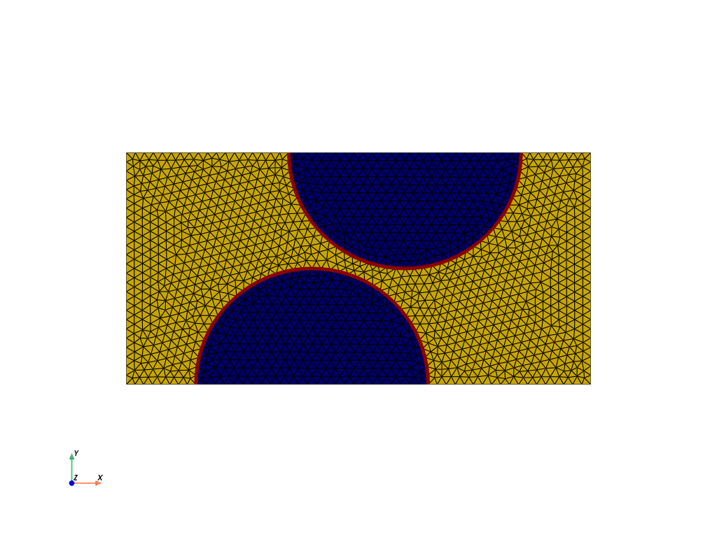
Each submesh is plotted individually:
plotter = pyvista.Plotter(off_screen=True)
grid1 = pyvista.UnstructuredGrid(*dolfinx.plot.vtk_mesh(subdomain1))
plotter.add_mesh(grid1, show_edges=True, color="gold")
grid2 = pyvista.UnstructuredGrid(*dolfinx.plot.vtk_mesh(subdomain2))
plotter.add_mesh(grid2, show_edges=True, color="darkblue")
gridi = pyvista.UnstructuredGrid(*dolfinx.plot.vtk_mesh(interface_mesh))
plotter.add_mesh(gridi, show_edges=True, color="darkred", line_width=5)
plotter.show_axes()
plotter.view_xy()
plotter.show()
Now that we have defined submeshes, we need to transfer (facets) meshtags from those defined on the original domain to their subdomain counterpart.
subdomain1_facet_tags, subdomain1_facet_map = transfer_meshtags_to_submesh(
    domain, facets, subdomain1, subdomain1_vertex_map, subdomain1_cell_map
)
subdomain2_facet_tags, subdomain2_facet_map = transfer_meshtags_to_submesh(
    domain, facets, subdomain2, subdomain2_vertex_map, subdomain2_cell_map
)
Entity map and integration measures#
Similarly to the previous CZM tour, entity maps must be defined to link integration of quantities defined on the subdomains.
cell_imap = domain.topology.index_map(tdim)
num_cells = cell_imap.size_local + cell_imap.num_ghosts
domain_to_subdomain1 = np.full(num_cells, -1, dtype=np.int32)
domain_to_subdomain1[subdomain1_cell_map] = np.arange(
    len(subdomain1_cell_map), dtype=np.int32
)
domain_to_subdomain2 = np.full(num_cells, -1, dtype=np.int32)
domain_to_subdomain2[subdomain2_cell_map] = np.arange(
    len(subdomain2_cell_map), dtype=np.int32
)

subdomain1.topology.create_connectivity(fdim, tdim)
subdomain2.topology.create_connectivity(fdim, tdim)

facet_imap = domain.topology.index_map(facets.dim)
num_facets = facet_imap.size_local + facet_imap.num_ghosts
domain_to_interface = np.full(num_facets, -1)
domain_to_interface[interface_cell_map] = np.arange(len(interface_cell_map))
Before setting up the entity_maps dictionary, we need a specific treatment for integrating terms on the interface. The interface_int_integration manually defines integration quantities on the interface. Besides, interface terms seen from one specific subdomain only exist on one side. As the assembler complains about this, there is a specific tweak to map cells from one side of the interface to the other side, thereby modifying the domain_to_subdomain maps. Moreover, we also consistently switch the orientation of the facets so that cells in subdomain 1 correspond to the "+" side of the interface and cells in subdomain 2 to the "-" side.
Note
Having a correct facet orientation does not really impact the results here as we do not distinguish between positive and negative opening of the cohesive zone in the formulation of the effective_opening. In case one wants to distinguish between positive and negative opening, an inconsistent facet orientation would produce incorrect results.
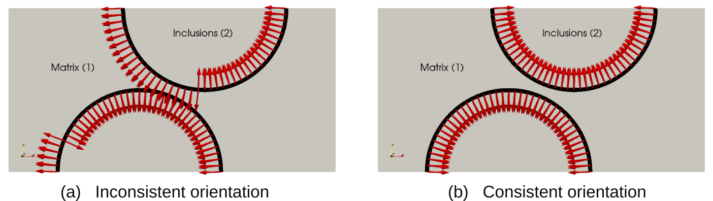
interface_entities, domain_to_subdomain1, domain_to_subdomain2 = interface_int_entities(
    domain, interface_facets, domain_to_subdomain1, domain_to_subdomain2
)

entity_maps = {
    interface_mesh: domain_to_interface,
    subdomain1: domain_to_subdomain1,
    subdomain2: domain_to_subdomain2,
}
We are now in position to define the various integration measures. The key point here is that the dInt interface measure is defined using prescribed integration entities which have been defined earlier. This is done by passing them to subdomain_data as follows.
dx = ufl.Measure("dx", domain=domain, subdomain_data=cells)
ds = ufl.Measure("ds", domain=domain, subdomain_data=facets)
dx_int = ufl.Measure("dx", domain=interface_mesh)
dInt = ufl.Measure(
    "dS",
    domain=domain,
    subdomain_data=[(INT_TAG, interface_entities)],
    subdomain_id=INT_TAG,
)
We can check that the length of the interface is properly computed.
Gamma = fem.assemble_scalar(fem.form(1 * dInt, entity_maps=entity_maps))
print(f"Check that Gamma is such that {Gamma} ~ {np.pi*2*radius}")
Check that Gamma is such that 1.570392630362744 ~ 1.5707963267948966
Weak form definition#
We generate a piecewise constant field of elastic properties, as in the previous tour.
E = create_piecewise_constant_field(domain, cells, {MATRIX_TAG: 3.09e3, INCL_TAG: 10e3})
nu = create_piecewise_constant_field(domain, cells, {MATRIX_TAG: 0.25, INCL_TAG: 0.4})
mu = E / (2.0 * (1.0 + nu))
lmbda = E * nu / ((1.0 + nu) * (1.0 - 2.0 * nu))


def epsilon(v):
    return ufl.sym(ufl.grad(v))


def sigma(v):
    return lmbda * ufl.tr(epsilon(v)) * ufl.Identity(tdim) + 2.0 * mu * epsilon(v)
Interfacial mechanical properties and expressions for the CZM law are defined similarly except that we consider constant properties since we define the CZM at the interface only.
Gc = fem.Constant(domain, 0.5)
sig_max = fem.Constant(domain, 50.0)
delta_0 = Gc / sig_max / ufl.exp(1)
beta = fem.Constant(domain, 2.0)


def normal_opening(v, n):
    return ufl.dot(v, n)


def tangential_opening(v, n):
    return v - normal_opening(v, n) * n


def effective_opening(v, n):
    return ufl.sqrt(normal_opening(v, n) ** 2 + beta**2 * tangential_opening(v, n) ** 2)


def T(opening, d):
    K_int = ufl.avg(Gc / delta_0**2) * (1 - d)
    return K_int * opening
In the previous tour, it was possible to use ufl.jump to define \(\jump{\bu}\). Here, we need to define it manually from two displacement fields u1 and u2 which live on two different subdomains. Here, we define \(\jump{\bu} = \bu^{(2)} - \bu^{(1)}\) where \((1)\) denotes subdomain 1 (the matrix) and \((2)\) denotes subdomain 2 (the inclusions). Note that we need to restrict quantities since we work with a facet measure. Although only one side exist for each subdomain, cells of a given subdomain from one side have been mapped to the other side, as discussed before. As a result, it does not really matter which side is used here. For consistency, we use the the "+" side for subdomain 1 and the "-" side for subdomain 2.
def jump(u1, u2):
    return u2("-") - u1("+")
We now define the relevant function spaces. As hinted before, the unknown \(\bu\) will consist of two displacements \((\bu^{(1)},\bu^{(2)})\) respectively belonging to a continuous Lagrange space defined on subdomains 1 and 2. We use a MixedFunctionSpace for this, meaning that we will end up with a block system. For easier post-processing, the computed displacement will be stored as a DG function, with jumps being non zero only at the interface.
V1 = fem.functionspace(subdomain1, ("Lagrange", 1, (tdim,)))
V2 = fem.functionspace(subdomain2, ("Lagrange", 1, (tdim,)))
W = ufl.MixedFunctionSpace(V1, V2)
u1 = fem.Function(V1, name="Displacement_1")
u2 = fem.Function(V2, name="Displacement_2")
v1, v2 = ufl.TestFunctions(W)
du1, du2 = ufl.TrialFunctions(W)
For easier post-processing, the computed displacement will be stored as a DG function, with jumps being non zero only at the interface. This space will not be used for defining the weak forms.
V = fem.functionspace(domain, ("DG", 1, (tdim,)))  # for post-processing only
u = fem.Function(V, name="Displacement")
Similarly to the previous tour, a DG-1 function space on the interface V_int will be used to represent the damage fields. Again, we could have used a Quadrature space but this choice proves easier for visualization purposes.
V_int = fem.functionspace(interface_mesh, ("DG", 1))
d = fem.Function(V_int, name="Interfacial_damage")
d_prev = fem.Function(V_int, name="Previous_interfacial_damage")
d_old = fem.Function(V_int, name="Interfacial_damage_old")
We can now define the expression for the interfacial damage based on the effective opening \(\delta\). The latter involves \(\jump{\bu}\) and the interface normal. Since \(\jump{\bu} = \bu^{(2)} - \bu^{(1)}\) , we need the normal \(\bn^{(1)\to(2)}\) from subdomain 1 to subdomain 2. This is n("+") since subdomain 1 is on "+" side of the interface and the facet normal points outwards the cell.
n1_to_2 = ufl.FacetNormal(domain)("+")
delta = effective_opening(jump(u1, u2), n1_to_2)
d_expr = ufl.max_value(ufl.avg(d_prev), 1 - ufl.exp(-delta / ufl.avg(delta_0)))
Bulk and interface contributions to the bilinear form are defined by separating the contributions of both subdomains.
a_bulk = ufl.inner(sigma(du1), epsilon(v1)) * dx(1) + ufl.inner(
    sigma(du2), epsilon(v2)
) * dx(2)
a_interface = ufl.dot(T(jump(du1, du2), ufl.avg(d)), jump(v1, v2)) * dInt
a = a_bulk + a_interface
f = fem.Constant(domain, np.zeros((tdim,)))
L = ufl.dot(f, v1) * dx(1) + ufl.dot(f, v2) * dx(2)
Finally, we use ufl.extract_blocks to obtain the different blocks \(\begin{bmatrix} \text{a}_{11} & \text{a}_{12}\\ \text{a}_{21} & \text{a}_{22}\end{bmatrix}\) of the bilinear form associated with \(\bu^{(1)}\) and \(\bu^{(2)}\). The blocked forms are then compiled by providing the entity maps.
a_blocked_compiled = fem.form(ufl.extract_blocks(a), entity_maps=entity_maps)
L_blocked_compiled = fem.form(ufl.extract_blocks(L), entity_maps=entity_maps)
As in the previous tour, we need to evaluate expressions that live on the facet mesh. We follow the same approach as discussed in details in Facet expressions interpolation.
q_p = V_int.element.interpolation_points()
weights = np.full(q_p.shape[0], 1.0)
q_el = basix.ufl.quadrature_element(
    interface_mesh.basix_cell(), scheme="custom", points=q_p, weights=weights
)
Q = fem.functionspace(interface_mesh, q_el)
q_ = ufl.TestFunction(Q)
dS_custom = ufl.Measure(
    "dS",
    domain=domain,
    metadata={
        "quadrature_scheme": "custom",
        "quadrature_points": q_p,
        "quadrature_weights": weights,
    },
    subdomain_data=[(INT_TAG, interface_entities)],
    subdomain_id=INT_TAG,
)

facet_interp = fem.form(
    1 / ufl.FacetArea(domain) * d_expr * ufl.avg(q_) * dS_custom,
    entity_maps=entity_maps,
)
Boundary conditions#
Dirichlet boundary conditions are now defined. Note that they involve only subdomain 1.
Uimp = fem.Constant(domain, (1.0, 0.0))
left_dofs = fem.locate_dofs_topological(V1, fdim, subdomain1_facet_tags.find(1))
right_dofs = fem.locate_dofs_topological(V1, fdim, subdomain1_facet_tags.find(2))

bcs = [
    fem.dirichletbc(np.zeros((tdim,)), left_dofs, V1),
    fem.dirichletbc(Uimp, right_dofs, V1),
]
The imposed displacement is initialized with unitary values so as to define the virtual displacement fields v_reac to be used for measuring the reaction force on the boundary in a consistent manner based on the equilibrium residual \(a(\bu,\bv_\text{read})-L(\bv_\text{reac})\).
v_reac1 = fem.Function(V1)
fem.set_bc(v_reac1.x.array, bcs)
v_reac2 = fem.Function(V2)
fem.set_bc(v_reac2.x.array, bcs)
virtual_work_form = fem.form(
    ufl.replace(a - L, {du1: u1, du2: u2, v1: v_reac1, v2: v_reac2}),
    entity_maps=entity_maps,
)
The linear problem associated with resolution of displacement at fixed damage is now defined outside the load-stepping loop. Since we use a mixed function space, we obtain a block linear system and therefore implement a custom class in utils.py for repeatedly solving a blocked linear variational problem. The latter expects blocked compiled linear and bilinear forms and a list of functions in which to store the results. The solver can be parametrized using PETSc options.
problem = BlockedLinearProblem(
    a_blocked_compiled,
    L_blocked_compiled,
    [u1, u2],
    bcs,
    petsc_options={
        "ksp_type": "preonly",
        "pc_type": "lu",
        "pc_factor_mat_solver_type": "mumps",
    },
)
Resolution#
The fixed-point resolution scheme is implemented as before. The main difference here lies in the post-processing steps. Data in u1 and u2 fields are transferred to a parent function u defined as a DG function on the parent mesh. We thus have a single displacement field in Paraview which presents jumps at the interface only.
Nincr = 40
loading = np.linspace(0, 0.04, Nincr + 1)


Niter_max = 200
tol = 1e-4
damage_results = [[0.0, 0.0]]
Force = [0.0]
iterations = [0]


out_file = io.VTKFile(MPI.COMM_WORLD, "results/czm.pvd", "a")
for i, t in enumerate(loading[1:]):
    print("Load step", i + 1)
    Uimp.value[0] = t
    nRes = 1.0
    j = 0
    while j < Niter_max:
        # displacement problem resolution
        problem.solve()
        # interpolation of damage on facets
        d.x.array[:] = fem.assemble_vector(facet_interp).array
        # normalized residual for convergence check
        nRes = (
            np.sqrt((fem.assemble_scalar(fem.form((d - d_old) ** 2 * dx_int)))) / Gamma
        )
        d_old.x.array[:] = d.x.array[:]
        j += 1
        print(f"    Iteration {j} | Residual: {nRes}")
        if nRes < tol:
            break
    else:
        raise ValueError(
            "Fixed-point solver did not converge in less than {} iterations".format(
                Niter_max
            )
        )
    iterations.append(j)
    d_prev.x.array[:] = d.x.array[:]

    Force.append(fem.assemble_scalar(virtual_work_form))

    # We interpolate both u1 and u2 into u for easier visualization with Paraview
    interpolate_submesh_to_parent(u, u1, subdomain1_cell_map)
    interpolate_submesh_to_parent(u, u2, subdomain2_cell_map)
    out_file.write_function(u, i)
    out_file.write_function(d, i)
    clear_output(wait=True)

out_file.close()
Load step 40
    Iteration 1 | Residual: 0.0017254351652441127
    Iteration 2 | Residual: 0.0011040370652327075
    Iteration 3 | Residual: 0.0005350765053613515
    Iteration 4 | Residual: 0.0002469718862936469
    Iteration 5 | Residual: 0.00011296609431889798
    Iteration 6 | Residual: 5.1586582223290735e-05
Results#
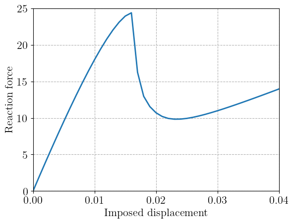
We finally plot the resulting load-displacement curve.
plt.figure()
plt.plot(loading, Force)
plt.xlabel("Imposed displacement")
plt.ylabel("Reaction force")
plt.show()