Elasto-plastic analysis of a 2D von Mises material #
Objectives
This demo shows how to implement a 2D elasto-plastic problem. Since the elasto-plastic behavior is isotropic with von Mises plasticity and linear hardening, the elasto-plastic constitutive update will have a closed-form analytical solution. We also implement a custom Newton nonlinear solver interacting with the constitutive update.
This demo works in parallel. \(\newcommand{\bsig}{\boldsymbol{\sigma}} \newcommand{\beps}{\boldsymbol{\varepsilon}} \newcommand{\bI}{\boldsymbol{I}} \newcommand{\CC}{\mathbb{C}} \newcommand{\bepsp}{\boldsymbol{\varepsilon}^\text{p}} \newcommand{\dev}{\operatorname{dev}} \newcommand{\tr}{\operatorname{tr}} \newcommand{\sigeq}{\sigma_\text{eq}} \newcommand{\bs}{\boldsymbol{s}}\)
Download sources
Problem position#
This example is concerned with the incremental analysis of an elasto-plastic von Mises material. The structure response is computed using an iterative predictor-corrector return mapping algorithm embedded in a Newton-Raphson global loop for restoring equilibrium. Due to the simple expression of the von Mises criterion, the return mapping procedure is completely analytical (with linear isotropic hardening).
Elastoplastic behavior#
The material is represented by an isotropic elasto-plastic von Mises yield condition of uniaxial strength \(\sigma_0\) and with isotropic hardening of modulus \(H\). The elastic behavior is linear isotropic:
The yield condition is given by:
where \(\bs = \dev(\bsig)\) is the deviatoric stress and \(p\) is the cumulated equivalent plastic strain which is such that \(\dot{p} = \sqrt{\frac{2}{3}}\|\dot{\beps}^\text{p}\|\). We also introduce the von Mises equivalent stress:
Plastic evolution is given by the associated flow rule:
which gives in the present case:
Predictor-corrector algorithm for constitutive behavior integration#
The return mapping procedure consists in finding a new stress \(\bsig_{n+1}\) and internal variable \(p_{n+1}\) state verifying the current plasticity condition from a previous stress \(\bsig_{n}\) and internal variable \(p_n\) state and an increment of total deformation \(\Delta \beps\). This step is quite classical in FEM plasticity for a von Mises criterion with isotropic hardening and follow notations from [Bonnet et al., 2014].
In the case of plastic flow, the flow rule (19) is approximated at \(t_{n+1}\) using a backward-Euler approximation:
An elastic trial stress \(\bsig_{\text{elas}} = \bsig_{n} + \CC:\Delta \beps\) is first computed. The plasticity criterion is then evaluated with the previous plastic strain \(f_{\text{elas}} = \sigeq^{\text{elas}} - \sigma_0 - H p_n\) where \(\sigeq^{\text{elas}}\) is the von Mises equivalent stress of the elastic trial stress.
If \(f_{\text{elas}} < 0\), no plasticity occurs during this time increment and \(\Delta p,\Delta \boldsymbol{\varepsilon}^p =0\) and \(\bsig_{n+1} = \bsig_\text{elas}\).
Otherwise, plasticity occurs and the increment of plastic strain \(\Delta p\) is such that:
Taking the deviatoric part of the first equation and injecting in the second shows that:
which results in:
Replacing in the third equation of (21), we deduce the value of the cumulated plastic strain increment:
and the plastic strain increment using the previous relations:
Hence, both elastic and plastic evolution can be accounted for by defining the plastic strain increment as follows:
where \(\langle \star \rangle_+\) denotes the positive part of \(\star\).
Implementation#
The considered problem is that of a plane strain hollow cylinder of internal (resp. external) radius \(R_i\) (resp. \(R_e\)) under internal uniform pressure \(q\).
We start by importing the relevant modules and define some geometrical constants.
import numpy as np
import matplotlib.pyplot as plt

import gmsh
from mpi4py import MPI
import ufl
import basix
from dolfinx import mesh, fem, io
import dolfinx.fem.petsc
from petsc4py import PETSc

hsize = 0.2

Re = 1.3
Ri = 1.0
We then model a quarter of cylinder using Gmsh similarly to the Axisymmetric formulation for elastic structures of revolution demo.
Show code cell source
gmsh.initialize()
gdim = 2
model_rank = 0
if MPI.COMM_WORLD.rank == 0:
    gmsh.option.setNumber("General.Terminal", 0)  # to disable meshing info
    gmsh.model.add("Model")

    geom = gmsh.model.geo
    center = geom.add_point(0, 0, 0)
    p1 = geom.add_point(Ri, 0, 0)
    p2 = geom.add_point(Re, 0, 0)
    p3 = geom.add_point(0, Re, 0)
    p4 = geom.add_point(0, Ri, 0)

    x_radius = geom.add_line(p1, p2)
    outer_circ = geom.add_circle_arc(p2, center, p3)
    y_radius = geom.add_line(p3, p4)
    inner_circ = geom.add_circle_arc(p4, center, p1)

    boundary = geom.add_curve_loop([x_radius, outer_circ, y_radius, inner_circ])
    surf = geom.add_plane_surface([boundary])

    geom.synchronize()

    gmsh.option.setNumber("Mesh.CharacteristicLengthMin", hsize)
    gmsh.option.setNumber("Mesh.CharacteristicLengthMax", hsize)

    gmsh.model.addPhysicalGroup(gdim, [surf], 1)
    gmsh.model.addPhysicalGroup(gdim - 1, [x_radius], 1, name="bottom")
    gmsh.model.addPhysicalGroup(gdim - 1, [y_radius], 2, name="left")
    gmsh.model.addPhysicalGroup(gdim - 1, [inner_circ], 3, name="inner")

    gmsh.model.mesh.generate(gdim)

domain, _, facets = io.gmshio.model_to_mesh(
    gmsh.model, MPI.COMM_WORLD, model_rank, gdim=gdim
)
gmsh.finalize()
We now define some material parameters and the function space for the displacement field. We choose here a standard \(\mathbb{P}_2\) Lagrange space.
E = fem.Constant(domain, 70e3)  # in MPa
nu = fem.Constant(domain, 0.3)
lmbda = E * nu / (1 + nu) / (1 - 2 * nu)
mu = E / 2.0 / (1 + nu)
sig0 = fem.Constant(domain, 250.0)  # yield strength in MPa
Et = E / 100.0  # tangent modulus
H = E * Et / (E - Et)  # hardening modulus


deg_u = 2
shape = (gdim,)
V = fem.functionspace(domain, ("P", deg_u, shape))
Attention
Elasto-plastic computations might result in volumetric locking issues induced by incompressible plastic deformations. In this demo, we do not attempt to solve this issue and use quadratic triangles which in 2D are sufficient to mitigate the locking phenomenon.
Boundary conditions correspond to symmetry conditions on the bottom and left parts (resp. numbered 1 and 2). Loading consists of a uniform pressure on the internal boundary (numbered 3). It will be progressively increased from 0 to a value slightly larger than \(q_\text{lim}=\dfrac{2}{\sqrt{3}}\sigma_0\log\left(\dfrac{R_e}{R_i}\right)\) which is the analytical collapse load for a perfectly-plastic material (no hardening).
Vx, _ = V.sub(0).collapse()
Vy, _ = V.sub(1).collapse()
bottom_dofsy = fem.locate_dofs_topological((V.sub(1), Vy), gdim - 1, facets.find(1))
top_dofsx = fem.locate_dofs_topological((V.sub(0), Vx), gdim - 1, facets.find(2))


# used for post-processing
def bottom_inside(x):
    return np.logical_and(np.isclose(x[0], Ri), np.isclose(x[1], 0))


bottom_inside_dof = fem.locate_dofs_geometrical((V.sub(0), Vx), bottom_inside)[0]

u0x = fem.Function(Vx)
u0y = fem.Function(Vy)
bcs = [
    fem.dirichletbc(u0x, top_dofsx, V.sub(0)),
    fem.dirichletbc(u0y, bottom_dofsy, V.sub(1)),
]

n = ufl.FacetNormal(domain)
q_lim = float(2 / np.sqrt(3) * np.log(Re / Ri) * sig0)

loading = fem.Constant(domain, 0.0)
Internal state variables and Quadrature elements#
When dealing with nonlinear constitutive models, internal state variables such as plastic strains represent the history seen by the material and have to be stored in some way. We choose here to represent them using Quadrature elements. This choice will make it possible to express the complex non-linear material constitutive equation at the Gauss points only, without involving any interpolation of non-linear expressions throughout the element. It will ensure an optimal convergence rate for the Newton-Raphson method, see chap. 26 of [Logg et al., 2012]. We will need Quadrature elements for 4-dimensional vectors and scalars, the number of Gauss points will be determined by the required degree deg_quad of the Quadrature element, see the Quadrature schemes tour for more details on the choice of quadrature rules.
Note
We point out that, although the problem is 2D, plastic strain still occur in the transverse \(zz\) direction. This will require us to keep track of the out-of-plane \(zz\) components of stress/strain states.
deg_quad = 2  # quadrature degree for internal state variable representation
W0e = basix.ufl.quadrature_element(
    domain.basix_cell(), value_shape=(), scheme="default", degree=deg_quad
)
We = basix.ufl.quadrature_element(
    domain.basix_cell(), value_shape=(4,), scheme="default", degree=deg_quad
)
W = fem.functionspace(domain, We)
W0 = fem.functionspace(domain, W0e)
Various functions are defined to keep track of the current internal state and currently computed increments.
sig = fem.Function(W)
sig_old = fem.Function(W)
n_elas = fem.Function(W)
beta = fem.Function(W0)
p = fem.Function(W0, name="Cumulative_plastic_strain")
dp = fem.Function(W0)
u = fem.Function(V, name="Total_displacement")
du = fem.Function(V, name="Iteration_correction")
Du = fem.Function(V, name="Current_increment")
v = ufl.TrialFunction(V)
u_ = ufl.TestFunction(V)

P0 = fem.functionspace(domain, ("DG", 0))
p_avg = fem.Function(P0, name="Plastic_strain")
Before writing the variational form, we now define some useful functions which will enable performing the constitutive relation update using the return mapping procedure described earlier. First, the strain tensor will be represented in a 3D fashion by appending zeros on the out-of-plane components since, even if the problem is 2D, the plastic constitutive relation will involve out-of-plane plastic strains. The elastic constitutive relation is also defined and a function as_3D_tensor will enable to represent a 4 dimensional vector containing respectively \(xx, yy, zz\) and \(xy\) components as a 3D tensor:
def eps(v):
    e = ufl.sym(ufl.grad(v))
    return ufl.as_tensor([[e[0, 0], e[0, 1], 0], [e[0, 1], e[1, 1], 0], [0, 0, 0]])


def elastic_behavior(eps_el):
    return lmbda * ufl.tr(eps_el) * ufl.Identity(3) + 2 * mu * eps_el


def as_3D_tensor(X):
    return ufl.as_tensor([[X[0], X[3], 0], [X[3], X[1], 0], [0, 0, X[2]]])


def to_vect(X):
    return ufl.as_vector([X[0, 0], X[1, 1], X[2, 2], X[0, 1]])
The return mapping procedure is implemented in the constitutive_update function which takes as an argument a total strain increment Δε, the previous stress state old_sig and the previous plastic strain old_p. For computing the plastic strain increment, we use formula (22) where ppos implements the positive part function.
Plastic evolution also requires the computation of the normal vector to the final yield surface given by \(\boldsymbol{n}_{\text{elas}} = \boldsymbol{s}_\text{elas}/\sigeq^{\text{elas}}\). In the following, this vector must be zero in case of elastic evolution. Hence, we multiply it by \(\dfrac{\langle f_{\text{elas}}\rangle_+}{ f_{\text{elas}}}\) to tackle both cases in a single expression. The final stress state is corrected by the plastic strain as follows \(\bsig_{n+1} = \bsig_{\text{elas}} - \beta \boldsymbol{s}_\text{elas}\) with \(\beta = \dfrac{3\mu}{\sigeq^{\text{elas}}}\Delta p\). It can be observed that the last term vanishes in case of elastic evolution so that the final stress is indeed the elastic predictor.
ppos = lambda x: ufl.max_value(x, 0)


def constitutive_update(Δε, old_sig, old_p):
    sig_n = as_3D_tensor(old_sig)
    sig_elas = sig_n + elastic_behavior(Δε)
    s = ufl.dev(sig_elas)
    sig_eq = ufl.sqrt(3 / 2.0 * ufl.inner(s, s))
    f_elas = sig_eq - sig0 - H * old_p
    dp = ppos(f_elas) / (3 * mu + H)
    n_elas = s / sig_eq * ppos(f_elas) / f_elas
    beta = 3 * mu * dp / sig_eq
    new_sig = sig_elas - beta * s
    return to_vect(new_sig), to_vect(n_elas), beta, dp
In order to use a Newton-Raphson procedure to resolve global equilibrium, we also need to derive the algorithmic consistent tangent matrix given by:
where \(\mathbb{Dev}\) is the 4th-order tensor associated with the deviatoric operator (note that \(\CC_{\text{tang}}^{\text{alg}}=\CC\) for elastic evolution). Contrary to what is done in [Logg et al., 2012], we do not store it as the components of a 4th-order tensor but it will suffice keeping track of the normal vector and the \(\beta\) parameter related to the plastic strains. We instead define the function sigma_tang computing the tangent stress \(\bsig_\text{tang} = \CC_{\text{tang}}^{\text{alg}}: \boldsymbol{\varepsilon}\) as follows:
def sigma_tang(eps):
    N_elas = as_3D_tensor(n_elas)
    return (
        elastic_behavior(eps)
        - 3 * mu * (3 * mu / (3 * mu + H) - beta) * ufl.inner(N_elas, eps) * N_elas
        - 2 * mu * beta * ufl.dev(eps)
    )
Attention
In this simple case, the stress expression from constitutive_update is explicit and can be represented using pure ufl expressions. Hence, we could use this nonlinear expression in the nonlinear residual and use automatic differentiation to compute directly the corresponding tangent form. Here, we voluntarily do differently, as a pedagogical way towards more complex constitutive models for which the stress expression is no longer explicit. In these cases, the stress and tangent stiffness have to be formally represented as quadrature points and the constitutive_update provides the corresponding values at quadrature points.
Global problem and custom Newton-Raphson procedure#
We now are in position to define the nonlinear residual variational form and the corresponding tangent bilinear form to be used in a global Newton-Raphson scheme. Each iteration will require establishing equilibrium by driving to zero the residual between the internal forces associated with the current stress state sig and the external force vector. Because we use Quadrature elements a custom integration measure dx must be defined to match the quadrature degree and scheme used by the Quadrature elements.
ds = ufl.Measure("ds", domain=domain, subdomain_data=facets)
dx = ufl.Measure(
    "dx",
    domain=domain,
    metadata={"quadrature_degree": deg_quad, "quadrature_scheme": "default"},
)
Residual = ufl.inner(eps(u_), as_3D_tensor(sig)) * dx - ufl.inner(
    -loading * n, u_
) * ds(3)
tangent_form = ufl.inner(eps(v), sigma_tang(eps(u_))) * dx
During the Newton-Raphson iterations, we will have to interpolate some ufl expressions at quadrature points to update the corresponding functions. We define the interpolate_quadrature function to do so. We first get the quadrature points location in the reference element and then use the fem.Expression.eval to evaluate the expression on all cells.
basix_celltype = getattr(basix.CellType, domain.topology.cell_type.name)
quadrature_points, weights = basix.make_quadrature(basix_celltype, deg_quad)

map_c = domain.topology.index_map(domain.topology.dim)
num_cells = map_c.size_local + map_c.num_ghosts
cells = np.arange(0, num_cells, dtype=np.int32)


def interpolate_quadrature(ufl_expr, function):
    expr_expr = fem.Expression(ufl_expr, quadrature_points)
    expr_eval = expr_expr.eval(domain, cells)
    function.x.array[:] = expr_eval.flatten()[:]
We now define the global Newton-Raphson loop. At each iteration, we need to solve a linear system of the form:
where \(\mathbf{R}\) is the current value of the nonlinear residual, \(\mathbf{du}\) the iteration correction to the unknown field \(\mathbf{u}\) and \(\mathbf{A}_\text{tang}\) the tangent operator of the nonlinear residual. To simplify the implementation, we rely on the fem.petsc.LinearProblem utility class to define and solve linear problems. In the following, we need to explicitly separate the steps where we assemble the linear system right-hand side from when we assemble the matrix left-hand side and solve the linear system. We therefore define a new class inheriting from LinearProblem and splitting these different steps.
Warning
We will use the CustomLinearProblem class within a custom implementation of the Newton method. During the course of the Newton iterations, we need to account for possible non-zero Dirichlet boundary conditions (although all Dirichlet boundary conditions are zero in the present case). We use the implementation provided in the FEniCSx Tutorial - Newton’s method with DirichletBC for lifting the right-hand side of the Newton system with non-zero Dirichlet boundary conditions.
class CustomLinearProblem(fem.petsc.LinearProblem):
    def assemble_rhs(self, u=None):
        """Assemble right-hand side and lift Dirichlet bcs.

        Parameters
        ----------
        u : dolfinx.fem.Function, optional
            For non-zero Dirichlet bcs u_D, use this function to assemble rhs with the value u_D - u_{bc}
            where u_{bc} is the value of the given u at the corresponding. Typically used for custom Newton methods
            with non-zero Dirichlet bcs.
        """

        # Assemble rhs
        with self._b.localForm() as b_loc:
            b_loc.set(0)
        fem.petsc.assemble_vector(self._b, self._L)

        # Apply boundary conditions to the rhs
        x0 = [] if u is None else [u.vector]
        fem.petsc.apply_lifting(self._b, [self._a], bcs=[self.bcs], x0=x0, scale=1.0)
        self._b.ghostUpdate(addv=PETSc.InsertMode.ADD, mode=PETSc.ScatterMode.REVERSE)
        x0 = None if u is None else u.vector
        fem.petsc.set_bc(self._b, self.bcs, x0, scale=1.0)

    def assemble_lhs(self):
        self._A.zeroEntries()
        fem.petsc.assemble_matrix_mat(self._A, self._a, bcs=self.bcs)
        self._A.assemble()

    def solve_system(self):
        # Solve linear system and update ghost values in the solution
        self._solver.solve(self._b, self._x)
        self.u.x.scatter_forward()


tangent_problem = CustomLinearProblem(
    tangent_form,
    -Residual,
    u=du,
    bcs=bcs,
    petsc_options={
        "ksp_type": "preonly",
        "pc_type": "lu",
        "pc_factor_mat_solver_type": "mumps",
    },
)
We discretize the applied loading using Nincr increments from \(0\) up to a value slightly larger than \(1\) (we exclude \(0\) from the list of load steps). A nonlinear discretization is adopted to refine the load steps during the plastic evolution phase. At each time increment, the system is assembled and the residual norm is computed. The incremental displacement Du is initialized to zero and the inner iteration loop performing the constitutive update is initiated. Inside this loop, corrections du to the displacement increment Du are computed by solving the Newton system and the return mapping update is performed using the current total strain increment deps. The resulting quantities are then interpolated onto their appropriate Quadrature function space. The Newton system and residuals are reassembled and this procedure continues until the residual norm falls below a given tolerance. After convergence of the iteration loop, the total displacement, stress and plastic strain states are updated for the next time step.
Nitermax, tol = 200, 1e-6  # parameters of the Newton-Raphson procedure
Nincr = 20
load_steps = np.linspace(0, 1.1, Nincr + 1)[1:] ** 0.5
results = np.zeros((Nincr + 1, 3))

# we set all functions to zero before entering the loop in case we would like to reexecute this code cell
sig.vector.set(0.0)
sig_old.vector.set(0.0)
p.vector.set(0.0)
u.vector.set(0.0)
n_elas.vector.set(0.0)
beta.vector.set(0.0)

Δε = eps(Du)
sig_, n_elas_, beta_, dp_ = constitutive_update(Δε, sig_old, p)


for i, t in enumerate(load_steps):
    loading.value = t * q_lim

    # compute the residual norm at the beginning of the load step
    tangent_problem.assemble_rhs()
    nRes0 = tangent_problem._b.norm()
    nRes = nRes0
    Du.x.array[:] = 0

    niter = 0
    while nRes / nRes0 > tol and niter < Nitermax:
        # solve for the displacement correction
        tangent_problem.assemble_lhs()
        tangent_problem.solve_system()

        # update the displacement increment with the current correction
        Du.vector.axpy(1, du.vector)  # Du = Du + 1*du
        Du.x.scatter_forward()

        # interpolate the new stresses and internal state variables
        interpolate_quadrature(sig_, sig)
        interpolate_quadrature(n_elas_, n_elas)
        interpolate_quadrature(beta_, beta)

        # compute the new residual
        tangent_problem.assemble_rhs()
        nRes = tangent_problem._b.norm()

        niter += 1

    # Update the displacement with the converged increment
    u.vector.axpy(1, Du.vector)  # u = u + 1*Du
    u.x.scatter_forward()

    # Update the previous plastic strain
    interpolate_quadrature(dp_, dp)
    p.vector.axpy(1, dp.vector)

    # Update the previous stress
    sig_old.x.array[:] = sig.x.array[:]

    if len(bottom_inside_dof) > 0:  # test if proc has dof
        results[i + 1, :] = (u.x.array[bottom_inside_dof[0]], t, niter)
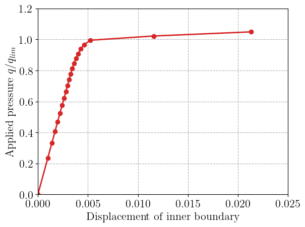
We plot the evolution e of the cylinder displacement on the inner boundary with the applied loading. We can check that we recover the correct analytical limit load when considering no hardening.
if len(bottom_inside_dof) > 0:  # test if proc has dof
    plt.plot(results[:, 0], results[:, 1], "-oC3")
    plt.xlabel("Displacement of inner boundary")
    plt.ylabel(r"Applied pressure $q/q_{lim}$")
    plt.show()
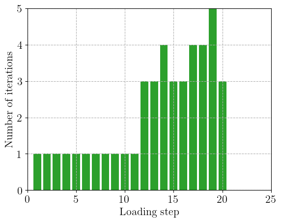
Finally, we also report the evolution of the number of Newton iterations as a function of the loading increments:
if len(bottom_inside_dof) > 0:
    plt.bar(np.arange(Nincr + 1), results[:, 2], color="C2")
    plt.xlabel("Loading step")
    plt.ylabel("Number of iterations")
    plt.xlim(0)
    plt.show()
References#
Marc Bonnet, Attilio Frangi, and Christian Rey. The finite element method in solid mechanics. McGraw-Hill Education New York, 2014. ISBN 978-8838674464.
Anders Logg, Kent-Andre Mardal, Garth N. Wells, and others. Automated Solution of Differential Equations by the Finite Element Method. Springer, 2012. ISBN 978-3-642-23098-1. doi:10.1007/978-3-642-23099-8.