Linear thermoelasticity (weak coupling)

Linear thermoelasticity (weak coupling) #

Introduction#

Objectives

In this tour, we will solve a linear thermoelastic problem. In permanent regime, the temperature field is uncoupled from the mechanical fields whereas the latter depend on the temperature due to presence of thermal strains in the thermoelastic constitutive relation. This situation can be described as weak thermomechanical coupling.

Download sources

Problem position#

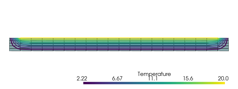
We consider the case of a rectangular 2D domain of dimensions $L \times H$ fully clamped on both lateral sides and subjected to a self-weight loading. The top side is subjected to a uniform temperature increase of $Δ T = + 20^{\circ} C$ while the bottom and lateral boundaries remain at the initial temperature $T_{0}$ . The geometry and boundary regions are first defined.

import numpy as np
import matplotlib.pyplot as plt
from mpi4py import MPI
import ufl
from dolfinx import fem, mesh, io, plot
import dolfinx.fem.petsc
import pyvista


L, H = 5, 0.3
Nx, Ny = 20, 5
domain = mesh.create_rectangle(
    MPI.COMM_WORLD,
    [(0.0, 0.0), (L, H)],
    [Nx, Ny],
    cell_type=mesh.CellType.quadrilateral,
)
gdim = domain.geometry.dim


def lateral_sides(x):
    return np.logical_or(np.isclose(x[0], 0.0), np.isclose(x[0], L))


def bottom(x):
    return np.isclose(x[1], 0.0)


def top(x):
    return np.isclose(x[1], H)

Because of the weak coupling discussed before, the thermal and mechanical problem can be solved separately. As a result, we don’t need to resort to mixed function spaces but can just define separately both problems.

Resolution of the thermal problem#

The temperature is solution to the following equation $div (k \nabla T) = 0$ where $k$ is the thermal conductivity (here we have no heat source). Since $k$ is assumed to be homogeneous, it will not influence the solution. We therefore obtain a standard Poisson equation without forcing terms. Its formulation and resolution in FEniCS is quite standard with the temperature variation $Δ T$ as the main unknown.

Note

We needed to define the linear form LT in order to use the LinearProblem utility class. We could also have equivalently defined the residual res = dot(grad(T), grad(T_))*dx and used the nonlinear utility class NonlinearProblem.

VT = fem.functionspace(domain, ("Q", 1))
T_, dT = ufl.TestFunction(VT), ufl.TrialFunction(VT)
Delta_T = fem.Function(VT, name="Temperature_variation")
aT = ufl.dot(ufl.grad(dT), ufl.grad(T_)) * ufl.dx
LT = fem.Constant(domain, 0.0) * T_ * ufl.dx

bot_dofs_T = fem.locate_dofs_geometrical(VT, bottom)
top_dofs_T = fem.locate_dofs_geometrical(VT, top)
sides_dofs_T = fem.locate_dofs_geometrical(VT, lateral_sides)
bcT = [
    fem.dirichletbc(0.0, bot_dofs_T, VT),
    fem.dirichletbc(20.0, top_dofs_T, VT),
    fem.dirichletbc(0.0, sides_dofs_T, VT),
]


# solve problem
problem = fem.petsc.LinearProblem(aT, LT, u=Delta_T, bcs=bcT)
problem.solve()

Coefficient(FunctionSpace(Mesh(blocked element (Basix element (P, quadrilateral, 1, gll_warped, unset, False, float64, []), (2,)), 0), Basix element (P, quadrilateral, 1, gll_warped, unset, False, float64, [])), 0)

We use pyvista to plot the corresponding temperature field:

pyvista.set_jupyter_backend("static")

topology, cell_types, geometry = plot.vtk_mesh(domain, gdim)
grid = pyvista.UnstructuredGrid(topology, cell_types, geometry)

T_topology, T_cell_types, T_geometry = plot.vtk_mesh(VT)
T_grid = pyvista.UnstructuredGrid(T_topology, T_cell_types, T_geometry)
T_grid.point_data["Temperature"] = Delta_T.x.array
T_grid.set_active_scalars("Temperature")
contours = T_grid.contour()

plotter = pyvista.Plotter()
plotter.window_size = (800, 300)
plotter.add_mesh(grid, show_edges=True)
plotter.add_mesh(contours, line_width=3)
plotter.view_xy()
plotter.zoom_camera(2.5)
plotter.show()

../../../_images/d5afeb1f2b12912e6db2a4850a490c13a01ec19112e96343df74a5aa412a4b5a.png

Mechanical problem#

The linearized thermoelastic constitutive equation is given by:

σ = C : (ε - α (T - T_{0}) 1) = λ tr (ε) 1 + 2 μ ε - α (3 λ + 2 μ) (T - T_{0}) 1

where $λ, μ$ are the Lamé parameters and $α$ is the thermal expansion coefficient. As regards the current problem, the last term corresponding to the thermal strains is completely known. The following formulation can thus be generalized to any kind of known initial stress or eigenstrain state such as pre-stress or phase changes.

Note

The weak formulation for the mechanical problem builds upon the presentation of the Linear elasticity tour. The main difference lies in the presence of the temperature term in the constitutive relation which introduces a linear term with respect to the TestFunction u_ when writing the work of internal forces ufl.inner(sigma(du, Delta_T), eps(u_)) * ufl.dx. As a result, the bilinear form is extracted using the left-hand side ufl.lhs function whereas the thermal strain term, acting as a loading term, is extracted using the right-hand side ufl.rhs function and added to the work of external forces when defining the linear form LM.

E = fem.Constant(domain, 50e3)
nu = fem.Constant(domain, 0.2)
mu = E / 2 / (1 + nu)
lmbda = E * nu / (1 + nu) / (1 - 2 * nu)
alpha = fem.Constant(domain, 1e-5)

f = fem.Constant(domain, (0.0, 0.0))


def eps(v):
    return ufl.sym(ufl.grad(v))


def sigma(v, Delta_T):
    return (
        lmbda * ufl.tr(eps(v)) - alpha * (3 * lmbda + 2 * mu) * Delta_T
    ) * ufl.Identity(gdim) + 2.0 * mu * eps(v)


Vu = fem.functionspace(domain, ("Q", 2, (gdim,)))
du = ufl.TrialFunction(Vu)
u_ = ufl.TestFunction(Vu)
Wint = ufl.inner(sigma(du, Delta_T), eps(u_)) * ufl.dx
aM = ufl.lhs(Wint)
LM = ufl.rhs(Wint) + ufl.inner(f, u_) * ufl.dx

lateral_dofs_u = fem.locate_dofs_geometrical(Vu, lateral_sides)
bcu = [fem.dirichletbc(np.zeros((gdim,)), lateral_dofs_u, Vu)]

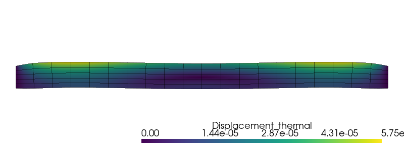
First, the self-weight loading is deactivated, only thermal stresses are computed.

u = fem.Function(Vu, name="Displacement")
problem = fem.petsc.LinearProblem(aM, LM, u=u, bcs=bcu)
problem.solve()

Coefficient(FunctionSpace(Mesh(blocked element (Basix element (P, quadrilateral, 1, gll_warped, unset, False, float64, []), (2,)), 0), blocked element (Basix element (P, quadrilateral, 2, gll_warped, unset, False, float64, []), (2,))), 1)

The deformed shape under thermal expansion is plotted using pyvista:

../../../_images/91c114313dbd7e8a7b0f56a9dd1a80e9408d93f0398410051201b77c29c6993c.png

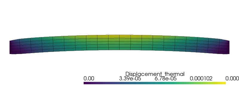
We now take into account the self-weight.

rho_g = 2400 * 9.81e-6
f.value[1] = -rho_g
problem.solve()

Coefficient(FunctionSpace(Mesh(blocked element (Basix element (P, quadrilateral, 1, gll_warped, unset, False, float64, []), (2,)), 0), blocked element (Basix element (P, quadrilateral, 2, gll_warped, unset, False, float64, []), (2,))), 1)

../../../_images/e4b7f26bb1717d128c0d3e4b15be5f073f58cc6abb35fc840f33634f15cb282b.png