Axisymmetric formulation for elastic structures of revolution

Axisymmetric formulation for elastic structures of revolution #

Objectives

This demo shows how to formulate a linear elastic problem under axisymmetric conditions. \(\newcommand{\bsig}{\boldsymbol{\sigma}} \newcommand{\beps}{\boldsymbol{\varepsilon}} \newcommand{\bu}{\boldsymbol{u}} \newcommand{\bv}{\boldsymbol{v}} \newcommand{\bT}{\boldsymbol{T}} \newcommand{\bI}{\boldsymbol{I}} \newcommand{\T}{^\text{T}} \newcommand{\tr}{\operatorname{tr}} \newcommand{\CC}{\mathbb{C}} \newcommand{\dOm}{\,\text{d}\Omega} \newcommand{\dom}{\,\text{d}\omega} \newcommand{\dS}{\,\text{d}S} \newcommand{\ds}{\,\text{d}s} \newcommand{\Neumann}{{\partial \Omega_\text{N}}} \newcommand{\Dirichlet}{{\partial \Omega_\text{D}}} \newcommand{\neumann}{{\partial \omega_\text{N}}} \newcommand{\dirichlet}{{\partial \omega_\text{D}}}\)

Download sources

../../../_images/axisymmetric_elasticity.png

We will consider a solid of revolution around a fixed axis \((Oz)\), the loading, boundary conditions and material properties being also invariant with respect to a rotation along the symmetry axis. The solid cross-section in a plane \(\theta=\text{cst}\) will be represented by a two-dimensional domain \(\omega\). With such a 2D mesh, the first spatial variable (x[0] in UFL) will represent the radial coordinate \(r\) whereas the second spatial variable (x[1]) will denote the axial variable \(z\).

Problem position#

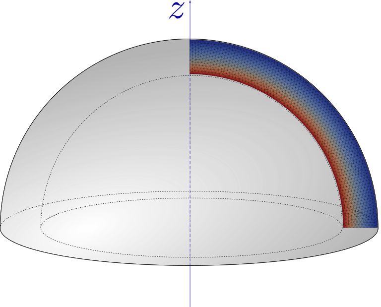
We will investigate here the case of a hollow hemisphere of inner (resp. outer) radius \(R_i\) (resp. \(R_e\)). We impose an external pressure on the outer radius boundary. Due to the revolution symmetry, the 2D cross-section corresponds to a quarter of a hollow cylinder.

We first import the relevant modules.

import numpy as np
import matplotlib.pyplot as plt

import gmsh
from mpi4py import MPI
import ufl
from dolfinx import mesh, fem, io
import dolfinx.fem.petsc

hsize = 0.2

Re = 11.0
Ri = 9.0

The domain is created and meshed using the Gmsh Python API.

Definition of axisymmetric strains and stresses#

For axisymmetric conditions, the unknown displacement field is of the form:

\[ \boldsymbol{u} = u_r(r,z)\boldsymbol{e}_r + u_z(r,z)\boldsymbol{e}_z \]

As a result, we will work with a standard vectorial function space of dimension 2 for discretizing \(u_r\) and \(u_z\) respectively. The associated strain components are however given by:

\[\begin{split} \boldsymbol{\varepsilon} = \begin{bmatrix} \partial_r u_r & 0 & (\partial_z u_r + \partial_r u_z)/2 \\ 0 & u_r/r & 0 \\ (\partial_z u_r + \partial_r u_z)/2 & 0 & \partial_z u_z\end{bmatrix}_{(\boldsymbol{e}_r,\boldsymbol{e}_\theta,\boldsymbol{e}_z)} \end{split}\]

The previous relation involves explicitly the radial variable \(r\), which can be obtained from the ufl.SpatialCoordinate x[0], the strain-displacement relation is then defined explicitly in the eps function.

Note

We could also express the strain components in the form of a vector of size 4 in alternative of the 3D tensor representation implemented below.

x = ufl.SpatialCoordinate(domain)


def eps(v):
    return ufl.sym(
        ufl.as_tensor(
            [
                [v[0].dx(0), 0, v[0].dx(1)],
                [0, v[0] / x[0], 0],
                [v[1].dx(0), 0, v[1].dx(1)],
            ]
        )
    )

The linear elastic constitutive equation giving the stress sigma is written using 3D tensors:

E = fem.Constant(domain, 1e5)
nu = fem.Constant(domain, 0.3)
mu = E / 2 / (1 + nu)
lmbda = E * nu / (1 + nu) / (1 - 2 * nu)


def sigma(v):
    return lmbda * ufl.tr(eps(v)) * ufl.Identity(3) + 2.0 * mu * eps(v)

Weak formulation#

The rest of the formulation is similar to the 2D elastic case with a small difference in the integration measure. Indeed, the virtual work principle reads as:

\[ \text{Find } \boldsymbol{u}\in V \text{ s.t. } \int_{\Omega} \boldsymbol{\sigma}(\boldsymbol{u}):\boldsymbol{\varepsilon}(\boldsymbol{v}) \dOm = \int_{\Neumann} \boldsymbol{T}\cdot\boldsymbol{v} \dS \quad \forall\boldsymbol{v} \in V \]

where \(\boldsymbol{T}\) is the imposed traction on some part \(\Neumann\) of the domain boundary.

In axisymmetric conditions, the full 3D domain \(\Omega\) can be decomposed as \(\Omega = \omega \times [0;2\pi]\) where the interval represents the \(\theta\) variable. The integration measures therefore reduce to \(\dOm = \dom\cdot(r\,\text{d}\theta)\) and \(\dS = \ds\cdot(r\,\text{d}\theta)\) where \(dS\) is the surface integration measure on the 3D domain \(\Omega\) and \(ds\) its counterpart on the cross-section boundary \(\partial \omega\). Exploiting the invariance of all fields with respect to \(\theta\), the previous virtual work principle is reformulated on the cross-section only as follows:

\[ \text{Find } \boldsymbol{u}\in V \text{ s.t. } \int_{\omega} \boldsymbol{\sigma}(\boldsymbol{u}):\boldsymbol{\varepsilon}(\boldsymbol{v}) r \dom = \int_{\neumann} \boldsymbol{T}\cdot\boldsymbol{v} r\ds \quad \forall\boldsymbol{v} \in V \]

where the \(2\pi\) constants arising from the integration on \(\theta\) have been cancelled on both sides. As a result, the bilinear and linear form are similar to the plane 2D case with the exception of the additional \(r\) term in the integration measures.

Warning

Some terms in the integrand, e.g. the strain \(\beps\), contain terms exhibiting a \(\dfrac{1}{r}\) singularity at \(r=0\). In practice, there should not be any issue regarding such a singularity since integrals are evaluated approximately using quadrature rules. Integrands are then evaluated at quadrature points which usually lie inside strictly inside the element (default scheme). For non-classical quadrature, such as vertex schemes or GLL points, you may have some trouble with such singular terms.

Resolution#

The final formulation is therefore pretty straightforward. Since a uniform pressure loading is applied on the outer boundary, we will also need the exterior normal vector to define the work of external forces form.

ds = ufl.Measure("ds", domain=domain, subdomain_data=facets)
dx = ufl.Measure("dx", domain=domain)

n = ufl.FacetNormal(domain)
p = fem.Constant(domain, 10.0)

V = fem.functionspace(domain, ("P", 2, (gdim,)))
du = ufl.TrialFunction(V)
u_ = ufl.TestFunction(V)
a_form = ufl.inner(sigma(du), eps(u_)) * x[0] * dx
L_form = ufl.inner(-p * n, u_) * x[0] * ds(3)

u = fem.Function(V, name="Displacement")

We apply smooth contact conditions on the vertical \(r=0\) (facet tag 2) and the horizontal \(z=0\) (facet tag 1) boundaries.

Vx, _ = V.sub(0).collapse()
Vy, _ = V.sub(1).collapse()
bottom_dofsy = fem.locate_dofs_topological((V.sub(1), Vy), gdim - 1, facets.find(1))
top_dofsx = fem.locate_dofs_topological((V.sub(0), Vx), gdim - 1, facets.find(2))

# used for post-processing
bottom_dofsx = fem.locate_dofs_topological((V.sub(0), Vx), gdim - 1, facets.find(1))[1]

u0x = fem.Function(Vx)
u0y = fem.Function(Vy)
bcs = [
    fem.dirichletbc(u0x, top_dofsx, V.sub(0)),
    fem.dirichletbc(u0y, bottom_dofsy, V.sub(1)),
]

# solve problem
problem = fem.petsc.LinearProblem(a_form, L_form, u=u, bcs=bcs)
problem.solve()

INFO: Disabling color, you really want to install colorlog.

Coefficient(FunctionSpace(Mesh(blocked element (Basix element (P, triangle, 1, equispaced, unset, False, float64, []), (2,)), 0), blocked element (Basix element (P, triangle, 2, gll_warped, unset, False, float64, []), (2,))), 0)

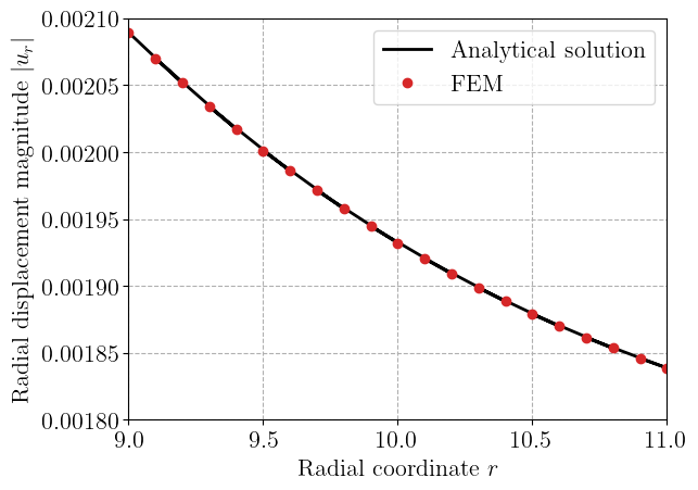
For this specific case, we can compare to the classical solution of a hollow sphere under external pressure with a purely radial displacement given by:

\[ u_r(r) = -\dfrac{R_e^3}{R_e^3-R_i^3}\left((1 − 2\nu)r + (1 + \nu)\dfrac{R_i^3}{2r^2}\right)\dfrac{p}{E}, \quad u_z=0 \]

We extract the radial displacement dofs on the bottom boundary and compare with the analytical solution.

ur = u.sub(0).collapse()
ur_FEM = ur.vector.array[bottom_dofsx]

r = Vx.tabulate_dof_coordinates()[bottom_dofsx, 0]

nu0 = nu.value
ur_theo = -(
    Re**3
    / (Re**3 - Ri**3)
    * float(p / E)
    * ((1 - 2 * nu0) * r + (1 + nu0) * Ri**3 / 2 / r**2)
)


plt.plot(r, np.abs(ur_theo), "-k", label="Analytical solution")
plt.plot(r, np.abs(ur_FEM), "oC3", label="FEM")
plt.xlabel("Radial coordinate $r$")
plt.ylabel("Radial displacement magnitude $|u_r|$")
plt.legend()
plt.show()

../../../_images/1364e0f57c98e97661afbca5a67bccd264a3b596a116bfcf14b6685e58b5c243.png